
GPU Gems 2
GPU Gems 2 is now available, right here, online. You can purchase a beautifully printed version of this book, and others in the series, at a 30% discount courtesy of InformIT and Addison-Wesley.
The CD content, including demos and content, is available on the web and for download.
Chapter 48. Medical Image Reconstruction with the FFT
Thilaka Sumanaweera
Siemens Medical Solutions USA
Donald Liu
Siemens Medical Solutions USA
In a number of medical imaging modalities, the Fast Fourier Transform (FFT) is being used for the reconstruction of images from acquired raw data. In this chapter, we present an implementation of the FFT in a GPU performing image reconstruction in magnetic resonance imaging (MRI) and ultrasonic imaging. Our implementation automatically balances the load between the vertex processor, the rasterizer, and the fragment processor; it also uses several other novel techniques to obtain high performance on the NVIDIA Quadro NV4x family of GPUs.
48.1 Background
The FFT has been implemented in GPUs before (Ansari 2003, Spitzer 2003, Moreland and Angel 2003). The improvements presented in this chapter, however, obtain higher performance from GPUs through numerous optimizations. In medical imaging devices used in computed tomography (CT), MRI, and ultrasonic scanning, among others, specialized hardware or CPUs are used to reconstruct images from acquired raw data. GPUs have the potential for providing better performance compared to the CPUs in medical image reconstruction at a cheaper cost, thanks to economic forces resulting from the large consumer PC market.
We review the Fourier transform and the classic Cooley-Tukey algorithm for the FFT and present an implementation of the algorithm for the GPU. We then present several specific approaches that we have employed for obtaining higher performance. We also briefly review the image-formation physics of MRI and ultrasonic imaging and present results obtained by reconstructing sample cine MRI and ultrasonic images on an NVIDIA Quadro FX NV40-based GPU using the FFT.
48.2 The Fourier Transform
The Fourier transform is an important mathematical transformation that is used in many areas of science and engineering, such as telecommunications, signal processing, and digital imaging. We briefly review the Fourier transform in this section. See Bracewell 1999 for a thorough introduction to Fourier transforms.
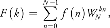
The Fourier transform of the 1D function f(x) is given by:
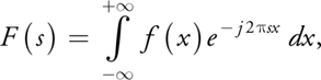
and the inverse Fourier transform is given by:
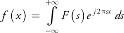
The Fourier transform can also be extended to 2, 3, . . ., N dimensions. For example, the 2D Fourier transform of the function f(x, y) is given by:
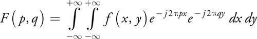
Note that the 2D Fourier transform can be carried out as two 1D Fourier transforms in sequence by first performing a 1D Fourier transform in x and then doing another 1D Fourier transform in y:
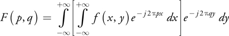
When processing digital signals, it is necessary to convert Equation 1 into a discrete form, turning the Fourier transform into a Discrete Fourier Transform (DFT):
where
is a set of discrete samples of a continuous signal and F(k), k = 0, . . ., N - 1, are the coefficients of its DFT. The inverse DFT is given by:
Note that both f(n) and  are complex numbers. When performing the DFT, F(k) is to be evaluated as shown in Equation 5 for all k, requiring N 2 complex multiplications and additions. However, the most widely used algorithm for computing the DFT is the FFT algorithm, which can perform the DFT using only N log2 N complex multiplications and additions, making it substantially faster, although it requires that N be a power of two. This algorithm is known as the Cooley-Tukey algorithm (Cooley and Tukey 1965), although it was also known to Carl Friedrich Gauss in 1805 (Gauss 1805, Heideman et al. 1984). We review this FFT algorithm in the next section.
48.3 The FFT Algorithm
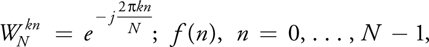
For simplicity, let us consider a discrete digital signal of eight samples: x(0), . . ., x(7). Figure 48-1 shows a flow chart of the FFT algorithm (the so-called decimation-in-time butterfly algorithm) for computing the DFT.
Figure 48-1 The Decimation-in-Time Butterfly Algorithm
On the left side of the figure, in Stage 1, the input samples are first sent through an input scrambler stage. If n is the index of the sample, that sample is sent to the kth output of the input scrambler, where
k = BIT_REVERSE(n)For example, sample index 3 (that is, 011 in binary) is sent to the output index (110 binary), which is 6. Every other output of the input scrambler is then multiplied by  , which has the value 1, and all outputs are sent to Stage 2. The input to Stage 2 is then scrambled again, multiplied by weights, and summed to generate the output of Stage 2. Each output of Stage 2 is generated by linearly combining two inputs. This process repeats for Stage 3 and Stage 4. The Fourier transform of the input signal is generated at the output of Stage 4.
In the more general case, if there are N input samples, there will be log2 N + 1 stages, requiring N log2 N complex multiplications and additions. The preceding algorithm can also be applied to do 2D, 3D, and ND FFTs. For example, consider an image, a 2D array of numbers. Using Equation 4, we could do a 1D FFT across all columns first and then do another 1D FFT across all rows to generate the 2D FFT.
48.4 Implementation on the GPU
The FFT can be implemented as a multipass algorithm. Referring to Figure 48-1, we observe that each stage can be implemented as a single pass in a fragment program. Note also that we can combine the input scrambler in Stage 1 and the scrambler in Stage 2 into a single stage (because is 1), an improvement over Ansari 2003 and Spitzer 2003. For our implementation, we make use of the following OpenGL extensions:
- WGL_ARB_pbuffer: We use a single pbuffer, with multiple draw buffers, as both the inputs and the outputs to each stage. Alternatively, we could have used one pbuffer as the input and another as the output to each stage. We chose the former method because it is slightly faster: using two pbuffers involves switching the rendering contexts, as in Ansari 2003.
- WGL_ARB_render_texture: The output of each stage is written to 2D textures for use as the input for the next stage.
- NV_float_buffer, NV_texture_rectangle: Used to create floating-point pbuffers and to input and output IEEE 32-bit floating-point numbers to and from each stage. The FFT operates on complex numbers. Furthermore, in applications such as MRI and ultrasonic imaging, it is important to use 32-bit floating-point numbers to obtain good numerical stability. Because of memory bandwidth limitations, looking up 32-bit floating-point scalars four times on a Quadro FX NV40-based GPU is faster than looking up a 32-bit floating-point four-vector once. Thus, it is advantageous to use GL_FLOAT_R32_NV texture internal format, instead of GL_FLOAT_RGBA32_NV format.
- ATI_texture_float: For certain texture lookups that do not require high precision (see the discussion later), two 16-bit floating-point numbers can be packed into a single 32-bit memory location using the GL_LUMINANCE_ALPHA_FLOAT16_ATI texture internal format.
- ATI_draw_buffers: Many modern GPUs support up to four render targets. Furthermore, on the Quadro FX NV4x family of GPUs, it is possible to create a pbuffer with eight draw buffers: GL_FRONT_LEFT, GL_BACK_LEFT, GL_FRONT_RIGHT, GL_BACK_RIGHT, GL_AUX0, GL_AUX1, GL_AUX2, and GL_AUX3, using the stereo mode. Using these two aspects, we can compute two FFTs in parallel by outputting two complex numbers to four render targets, and then use those four render targets as input to the next stage—without having to switch contexts, as is the case when using two separate pbuffers.
- ARB_fragment_program: The weights, , can be computed inside the fragment program using a single SCS instruction, as discussed in Section 48.4.2.
The application first creates a single GL_FLOAT_R32_NV floating-point stereo pbuffer. Note that the stereo mode must be enabled from the control panel for this to be effective. The pbuffer comes with eight 32-bit scalar draw buffers:
- GL_FRONT_LEFT
- GL_BACK_LEFT
- GL_FRONT_RIGHT
- GL_BACK_RIGHT
- GL_AUX0
- GL_AUX1
- GL_AUX2
- GL_AUX3
In the first pass, GL_FRONT_LEFT, GL_BACK_LEFT, GL_FRONT_RIGHT, and GL_BACK_RIGHT are the source draw buffers, and GL_AUX0, GL_AUX1, GL_AUX2, and GL_AUX3 are the destination draw buffers. GL_FRONT_LEFT and GL_AUX0 contain the real part of the first FFT, while GL_BACK_LEFT and GL_AUX1 contain the imaginary part of the first FFT. GL_FRONT_RIGHT and GL_AUX2 contain the real part of the second FFT, while GL_BACK_RIGHT and GL_AUX3 contain the imaginary part of the second FFT. In subsequent passes, the source and destination draw buffers are swapped and the process continues. After all the stages are complete, what are remaining in the destination draw buffers are the FFTs of the two input 2D data arrays. The application then displays the magnitude of the FFT for one of the data arrays.
We employ two approaches: (1) mostly loading the fragment processor and (2) loading the vertex processor, the rasterizer, and the fragment processor. We present the advantages and limitations of the two approaches and discuss a way to use a combination of the two to obtain the best performance from a Quadro NV40 GPU.
48.4.1 Approach 1: Mostly Loading the Fragment Processor
In this approach, the application renders a series of quads covering the entire 2D data array, parallel to the pbuffer for each stage of the algorithm. The application also creates a series of 1D textures, called butterfly lookups, required for each stage for scrambling the input data and for looking up . Naturally, the scrambling indices are integers. The largest possible index when pbuffers are used is 2048, the size of the largest texture that can be created in an NV40-based Quadro FX. This means we can use 16-bit precision to store these indices. Because there are two indices to look up, we can pack two 16-bit indices into a single 32-bit memory location of a texture with the GL_LUMINANCE_ALPHA_FLOAT16_ATI internal format. This way, a single texture lookup can generate both scrambling indices. As for the weights, , we use two separate GL_FLOAT_R32_NV textures to store the real and imaginary parts of them.
A fragment program is executed for each sample of the data array. In this approach, the fragment processor is the bottleneck. The vertex processor and the rasterizer are idling for the most part, because there is just a single quad drawn for each stage. Listing 48-1 shows the Cg fragment program for this case.
Example 48-1. Cg Fragment Program for a Single Stage of the FFT (Approach 1)
void FragmentProgram(in float4 TexCoordRect
                     : TEXCOORD0, out float4 sColor0
                     : COLOR0, out float4 sColor1
                     : COLOR1, out float4 sColor2
                     : COLOR2, out float4 sColor3
                     : COLOR3, uniform samplerRECT Real1,
                       uniform samplerRECT Imag1, uniform samplerRECT Real2,
                       uniform samplerRECT Imag2,
                       uniform samplerRECT ButterflyLookupI,
                       uniform samplerRECT ButterflyLookupWR,
                       uniform samplerRECT ButterflyLookupWI)
{
  float4 i = texRECT(ButterflyLookupI, TexCoordRect.xy);
  // Read in scrambling
  // coordinates
  float4 WR = texRECT(ButterflyLookupWR, TexCoordRect.xy);
  // Read in weights
  float4 WI = texRECT(ButterflyLookupWI, //
                      TexCoordRect.xy);
  float2 Res;
  float2 r1 = float2(i.x, TexCoordRect.y);
  float2 r2 = float2(i.w, TexCoordRect.y);
  float4 InputX1 = texRECT(Real1, r1);
  float4 InputY1 = texRECT(Imag1, r1);
  float4 InputX2 = texRECT(Real1, r2);
  float4 InputY2 = texRECT(Imag1, r2);
  Res.x = WR.x * InputX2.x - WI.x * InputY2.x;
  Res.y = WI.x * InputX2.x + WR.x * InputY2.x;
  sColor0.x = InputX1.x + Res.x;
  // Output data array 1
  sColor1.x = InputY1.x + Res.y;
  //
  float4 InputX1_ = texRECT(Real2, r1);
  float4 InputY1_ = texRECT(Imag2, r1);
  float4 InputX2_ = texRECT(Real2, r2);
  float4 InputY2_ = texRECT(Imag2, r2);
  Res.x = WR.x * InputX2_.x - WI.x * InputY2_.x;
  Res.y = WI.x * InputX2_.x + WR.x * InputY2_.x;
  sColor2.x = InputX1_.x + Res.x;
  // Output data array 2
  sColor3.x = InputY1_.x + Res.y;
  //
}
The input to this program is the texture coordinates of the data sample, TexCoordRect, and the outputs are the render targets: sColor0 through sColor3. The uniform variables (Real1, Imag1) are the real and imaginary parts of the first 2D data array and (Real2, Imag2) the real and imaginary parts of the second 2D data array. The uniform variable ButterflyLookupI contains the scrambling coordinates. The uniform variables ButterflyLookupWR and ButterflyLookupWI contain the real and imaginary parts of the weights.
Lines 1–3 of Listing 48-1 read in the coordinates, i, for scrambling the input data samples and the real and imaginary parts of the weights (WR and WI) for combining the two inputs. The variables r1 and r2 contain the coordinates for looking up the data values, InputX1, InputY1, InputX2, and InputY2. Lines 13 and 14 compute the output values for the first 2D data array, while lines 21 and 22 compute the output values for the second 2D data array.
As mentioned earlier, the vertex processor and the rasterizer are idling for the most part in this approach. If we moved more computing load to the vertex processor and the rasterizer, we might improve the performance for some cases. We do just that in the second approach.
48.4.2 Approach 2: Loading the Vertex Processor, the Rasterizer, and the Fragment Processor
Figure 48-2 shows an alternate representation of Figure 48-1. Each circle corresponds to a fragment in a given pass. Shown in square brackets are the two scrambling indices used by the fragment program. Also shown is the weight, , used by the fragment program. For each stage, groups of fragments are lumped together to form contiguous blocks, shown in blue and green. It can be observed that for each block, the scrambling indices and the angular argument of the weight, 2k/N, vary linearly. What this means is that instead of drawing a single quad covering the entire 2D data array, if we draw a series of smaller quads corresponding to each block and let the vertex processor interpolate the scrambling indices and the angular argument, we should be able to move some load off of the fragment processor into the vertex processor and the rasterizer. Listing 48-2 shows the Cg fragment program for Approach 2.
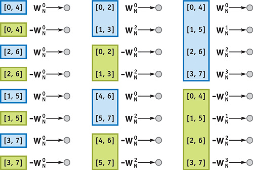
Figure 48-2 Another Way to Represent the Decimation-in-Time Butterfly Algorithm
Example 48-2. Cg Fragment Program for a Single Stage of the FFT (Approach 2)
void FragmentProgram(in float4 TexCoordRect0
                     : TEXCOORD0, in float4 TexCoordRect1
                     : TEXCOORD1, out float4 sColor0
                     : COLOR0, out float4 sColor1
                     : COLOR1, out float4 sColor2
                     : COLOR2, out float4 sColor3
                     : COLOR3, uniform samplerRECT Real1,
                       uniform samplerRECT Imag1, uniform samplerRECT Real2,
                       uniform samplerRECT Imag2)
{
  float4 WR;
  float4 WI;
  float4 i0 = float4(TexCoordRect0.z, 0.0, 0.0, 0.0); // Scrambling
  // coordinates
  float4 i1 = float4(TexCoordRect0.w, 0.0, 0.0, 0.0); //
  sincos(TexCoordRect1.x, WI.x, WR.x);
  // Compute
  // weights
  float2 Res;
  float2 r1 = float2(i0.x, TexCoordRect.y);
  float2 r2 = float2(i1.x, TexCoordRect.y);
  float4 InputX1 = texRECT(Real1, r1);
  float4 InputY1 = texRECT(Imag1, r1);
  float4 InputX2 = texRECT(Real1, r2);
  float4 InputY2 = texRECT(Imag1, r2);
  Res.x = WR.x * InputX2.x - WI.x * InputY2.x;
  Res.y = WI.x * InputX2.x + WR.x * InputY2.x;
  sColor0.x = InputX1.x + Res.x;
  // Output data array 1
  sColor1.x = InputY1.x + Res.y;
  //
  float4 InputX1_ = texRECT(Real2, r1);
  float4 InputY1_ = texRECT(Imag2, r1);
  float4 InputX2_ = texRECT(Real2, r2);
  float4 InputY2_ = texRECT(Imag2, r2);
  Res.x = WR.x * InputX2_.x - WI.x * InputY2_.x;
  Res.y = WI.x * InputX2_.x + WR.x * InputY2_.x;
  sColor2.x = InputX1_.x + Res.x;
  // Output data array 2
  sColor3.x = InputY1_.x + Res.y;
  //
}
Notice that compared to Listing 48-1, the butterfly lookup texture uniform variables are now missing. The inputs to this program are the texture coordinates of the data sample, TexCoordRect0 and TexCoordRect1. The values of TexCoordRect0.z and TexCoordRect0.w contain the scrambling coordinates, and the value of TexCoordRect1.x contains the angular argument, all interpolated by the rasterizer. Note also that in line 5 of the body of the program, the weights WR and WI are computed by calling the sincos instruction.
48.4.3 Load Balancing
Notice also that for later stages of Approach 2, the number of quads we have to draw is only a handful. For the early stages, the number of quads we have to draw is quite large. For example, for Stage 1, we need to draw one quad for each fragment. This means that the vertex processor and the rasterizer can become the bottleneck for early stages, resulting in performance degradation worse than that of Approach 1.
However, it is possible to use Approach 1 for the early stages and Approach 2 for the later stages and reach an overall performance better than using Approaches 1 or 2 alone. The accompanying software automatically chooses the transition point by trying out all possible transition points and picking the one with the best performance.
48.4.4 Benchmarking Results
Table 48-1 compares the performance of our 2D FFT implementation with optimized 2D FFT implementations available in the FFTW library (http://www.fftw.org). For the NV40-based Quadro FX, two 2D images were uploaded once into the GPU's video memory and then Fourier-transformed continuously. All inputs and outputs were 32-bit IEEE numbers. The FFTW_PATIENT mode of the FFTW library was used; this mode spends some time when the library is initialized choosing the fastest CPU implementation. The second column lists the frame rates reached using Approach 1 alone, while the third column lists the frame rates reached using load balancing. The fourth column lists the frame rates for using the CPU, and the fifth column shows the frame rate gain of using load balancing on the GPU over using the CPU. All results were acquired on an NVIDIA Quadro FX 4000 using driver 7.0.4.1 (beta), released on October 9, 2004. Notice that in all cases, the GPU outperformed the CPU. We saw the largest gain over the CPU for a 2048x64 2D image, reaching a factor of 1.97.
Table 48-1. Comparing GPU and CPU Performance
|
Image Size |
Fragment Processor Only |
Vertex and Fragment Processors |
FFTW |
Gain over CPU |
|
256x256 |
430 |
473 |
355 |
1.33 |
|
512x512 |
95 |
104 |
56 |
1.86 |
|
2048x32 |
387 |
426 |
230 |
1.85 |
|
2048x64 |
190 |
207 |
105 |
1.97 |
|
2048x128 |
91 |
100 |
53 |
1.89 |
|
2048x256 |
44 |
48 |
26 |
1.85 |
|
2048x512 |
21 |
23 |
13 |
1.77 |
|
2048x1024 |
10 |
11 |
6 |
1.83 |
|
1024x256 |
93 |
102 |
54 |
1.89 |
|
1024x512 |
45 |
49 |
27 |
1.81 |
48.5 The FFT in Medical Imaging
The FFT is a heavily used mathematical tool in medical imaging. A number of medical imaging modalities, such as CT, MRI, and ultrasonic imaging, rely on the FFT to generate images of the human anatomy from the acquired raw data. We look at MRI and ultrasonic imaging in more detail here. See Bushberg et al. 2001 for an excellent in-depth review of the basics of CT, MRI, and ultrasonic imaging.
48.5.1 Magnetic Resonance Imaging
We review MRI image formation physics very briefly in this section. A more thorough introduction to MRI can be found in Liang and Lauterbur 2000. The density of protons, or hydrogen (1H) atoms, in the human body can be imaged using MRI. The human body contains primarily water, carrying large quantities of protons. The behavior of the protons is governed by the principles of quantum mechanics. However, we can use principles from classical mechanics to explain the process of forming images using MRI more intuitively.
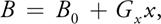
Consider a 1D object, for simplicity. The protons in the object can be thought of as tiny magnets, with magnetism produced by spinning charged particles. In the absence of an external magnetic field, these tiny magnets are randomly oriented, thus displaying no preferred direction of magnetization. If the object is placed in a strong magnetic field, B 0, on the order of 1 Tesla, the majority of these tiny magnets will align along the magnetic field and will spin at a rate given by:

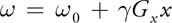
where is the gyromagnetic ratio for 1H and 0 is called the Larmor frequency. An MRI scanner contains a strong constant magnetic field, superimposed on linear magnetic gradients. If the magnetic field B varies linearly across the field of view as:
then the Larmor frequency varies linearly as:
Without going into more detail, it is possible to collect a signal from the object sitting in this magnetic field by exciting the tissue with a radio frequency (RF) pulse and listening to the echo, using an antenna or a coil. The received RF signal is given by:
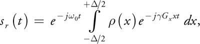
where, (x) is the proton density, is the extent of our 1D object, sr (t) is the received signal from the tissue, and t is time, which corresponds to the Fourier spatial-frequency dimension of the object. Equation 10 shows an amplitude-modulated signal on a carrier tone with an angular frequency, 0. After amplitude demodulation, the received signal is:
Equation 11 shows that the collected data is the Fourier transform of the proton density of the object. Hence the proton density, (x), of the object can be reconstructed by performing an inverse Fourier transform on the acquired signal.
Equation 11 can be thought of as "traversing" the Fourier spatial-frequency space as time changes. When time is zero, we are at the origin of the Fourier domain. As time increases, we are at high frequencies. Equation 11 shows only 1D MRI imaging, but it can be extended to do 2D and 3D MRI imaging as well. Briefly, in 2D MRI imaging, a slice through the object is imaged by first selectively exciting the desired slice of tissue and then traversing the Fourier spatial-frequency space in 2D, line by line:
where the spatial-frequency space is given by (t, ty ), Gy is the y gradient of the magnetic field, and (x, y) is the 2D proton density of the object. Once again, (x, y) can be reconstructed from the acquired data by doing a 2D inverse Fourier transform.
48.5.2 Results in MRI
In this section, we present some examples of MRI images reconstructed using the GPU.
Example 1: Mouse Heart
Figure 48-3a shows the acquired Fourier space data and Figure 48-3b the reconstructed data of a mouse heart.[1] The AVI file named MouseOut.avi on the book's CD shows the beating heart of the mouse, although the playback speed of the movie is slowed to 15 Hz to facilitate viewing, down significantly from the actual data acquisition rate, 127 Hz. This movie contains 13 frames and was acquired using 192 cardiac cycles, with each cycle acquiring 13 Fourier-space raster lines corresponding to different frames. The temporal sampling rate between frames is 7.9 ms (127 Hz). The inputs to the GPU were two floating-point 256x256 arrays containing real and imaginary parts of the data. The GPU reconstructed this data at 172 Hz on a 2.5 GHz Pentium 4, AGP 4x PC. This frame rate includes the time to upload the data over the AGP bus.
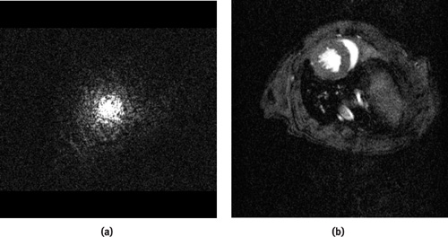
Figure 48-3 Images Generated from MRI Data
The book's CD contains the original raw data in Fourier space and a program demonstrating the use of the GPU for reconstructing the data.
Example 2: Human Head
Figure 48-4a shows the acquired Fourier space data and Figure 48-4b the reconstructed data of a human head. [2] The AVI file named HeadOut.avi on the book's CD shows 16 axial slices through the head, played as a movie. Again, the inputs to the GPU were two floating-point 256x256 arrays containing real and imaginary parts of the data.
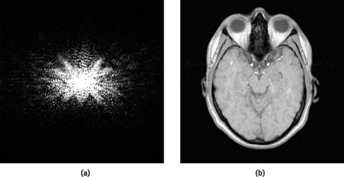
Figure 48-4 Data from a Human Head
The book's CD contains the original raw data in Fourier space and a program demonstrating the use of the GPU for reconstructing the data.
48.5.3 Ultrasonic Imaging
Traditional ultrasonic imaging does not make use of the FFT for image formation, but rather uses a time-domain delay-sum data-processing approach for beam forming. Beam forming is the process of forming an image by firing and receiving ultrasonic pulses into an object. See Wright 1997 for an introduction to traditional ultrasonic beam forming. In this section, we describe a new method called pulse plane-wave imaging (PPI) for forming images using the FFT (Liu 2002), which has the advantage of reaching frame rates an order of magnitude higher than those reachable by traditional ultrasonic imaging.
Figure 48-5a shows an ultrasonic transducer, containing an array of N piezoelectric elements. Each piezoelectric element is connected to a channel containing a transmitter and is capable of transmitting an ultrasonic pulse such as the one shown in Figure 48-5b with frequencies on the order of 1 to 20 MHz. The transducer (with a layer of coupling gel) is placed on the body for imaging the human anatomy. In traditional beam forming, ultrasound beams are fired into the body starting from one end of the transducer to the other end, acquiring an image line by line, just as is done in radar imaging.
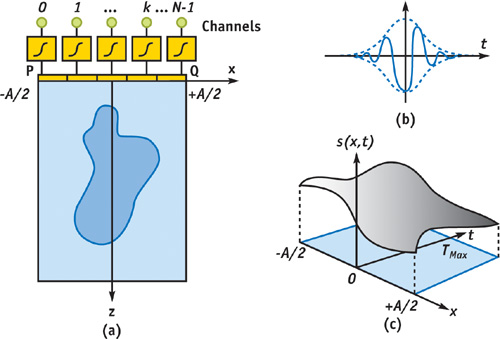
Figure 48-5 Ultrasonic Imaging Using PPI
In the PPI approach, all the elements are pulsed at the same time, producing a single plane-wave front oriented along the z axis, illuminating the entire field of view to be scanned. Immediately after the pulse is sent, the piezoelectric elements are switched to a set of receive circuitry in the channel. The signal received by each element in the array is sent to a receive amplifier and then on to an analog-to-digital converter in the channel. For simplicity, let's assume that the array is a continuous function. Figure 48-5c shows the signal, s(x, t), recorded by all elements within x  [-A/2, + A/2] for t [0, T max]. Let the ultrasonic scattering coefficient at a point be (x, z). Our goal is to reconstruct the scattering coefficient using s(x, t). As can be seen from the appendix on the book's CD, the 2D Fourier transform of the scattering coefficient is given by:
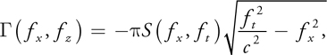
where
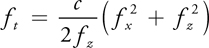
and S(fx , ft ) is the 2D Fourier transform of s(x, t). Equations 1313 and 14 show the gist of ultrasonic image formation using pulse plane-wave imaging. The scattering coefficient can be reconstructed by using the following steps:
- Send a plane wave into the body and record the returned signal, s(x, t).
- Do a 2D Fourier transform on the returned signal to produce S(fx , ft ).
- Remap the values of ft frequencies in S(fx , ft ) using Equation 13 to produce (fx , fz ).
- Perform an inverse 2D Fourier transform on (fx , fz ) to produce (x, z).
Figure 48-6 shows these four steps diagrammatically. The 2D FFT and 2D IFFT can be implemented on the GPU as shown in Section 48.4. The frequency remapping between steps 2 and 3 can also be easily implemented on the GPU. Figure 48-7 shows a block diagram of the pipeline of processing the ultrasound data.
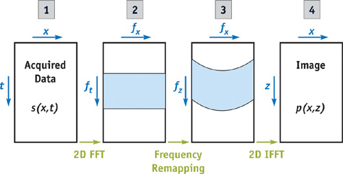
Figure 48-6 The Steps in Forming an Ultrasonic Image Using PPI
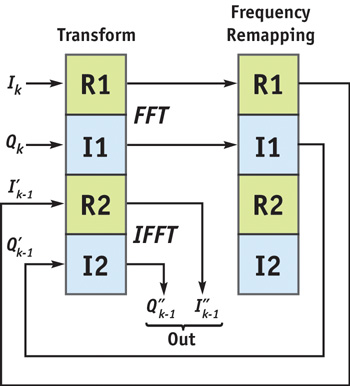
Figure 48-7 The Processing Pipeline for Reconstructing Ultrasound Data
The [R1, I1] channels perform the FFT, while [R2, I2] channels perform the IFFT in each transform step. Note that the algorithm for the IFFT is the same as that for the FFT, except for a change in sign for the angular argument of the weight. At the kth iteration, we are inputting the acquired data (Ik , Qk ) to the [R1, I1] channels for undergoing the FFT. The output of this step is then sent to the frequency-remapping step, which essentially warps the Fourier domain data along ft . The [R1, I1] output of this step is then sent to the [R2, I2] input of the transform step, which does the IFFT on [R2, I2] and the FFT on the next input frame of data in [R1, I1]. The [R2, I2] output of the transform step then contains the reconstructed image data.
Results in Ultrasonic Imaging
Figure 48-8a shows the acquired data of a simulated phantom containing four point targets, and Figure 48-8b shows the resulting phantom image after processing using steps 1–4. Notice that the point targets can be resolved well in the reconstructed image. The frame rate of the PPI approach is at least an order of magnitude faster than the traditional delay-sum beam-forming approach.
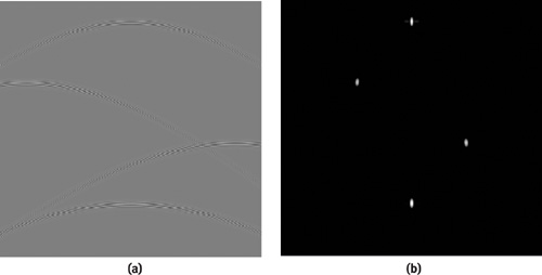
Figure 48-8 Simulated and Reconstructed Data of a Phantom
48.6 Conclusion
We presented an optimized implementation of the 2D FFT on an NV40-based Quadro FX GPU, as well as its application in MRI and ultrasonic imaging for image reconstruction. We also presented a new method for ultrasonic beam forming, which is more amenable to an implementation in the GPU. The performance of the GPU for the 2D FFT is better than that of a 2.5 GHz Pentium 4 CPU for all cases we tested. For some cases, the performance of the GPU was close to a factor of two better than the CPU's performance.
Besides the performance advantage of using a GPU over a CPU for medical image reconstruction, there are other advantages as well. In a medical imaging device, the CPU can be preoccupied with time-critical tasks such as controlling the data acquisition hardware. In this case, it is advantageous to use the GPU for image reconstruction, leaving the CPU to do data acquisition. Furthermore, unlike the CPU, the GPU is free of interrupts from the operating system, resulting in more predictable behavior. The rate of increase in performance of GPUs is expected to surpass that of CPUs in the next few years, increasing the appeal of the GPU as the processor of choice for medical image reconstruction.
48.7 References
Ansari, Marwan. 2003. "Video Image Processing Using Shaders." Presentation at Game Developers Conference 2003.
Bracewell, Ronald N. 1999. The Fourier Transform and Its Applications. McGraw-Hill.
Bushberg, Jerrold T., J. Anthony Seibert, Edwin M. Leidholdt, Jr., and John M. Boone. 2001. The Essential Physics of Medical Imaging, 2nd ed. Lippincott Williams & Wilkins.
Cooley, James W., and John Tukey. 1965. "An Algorithm for the Machine Calculation of Complex Fourier Series." Mathematics of Computation 19, pp. 297–301.
Gauss, Carl F. 1805. "Nachlass: Theoria Interpolationis Methodo Nova Tractata." Werke 3, pp. 265–327, Königliche Gesellschaft der Wissenschaften, Göttingen, 1866.
Heideman, M. T., D. H. Johnson, and C. S. Burrus. 1984. "Gauss and the History of the Fast Fourier Transform." IEEE ASSP Magazine 1(4), pp. 14–21.
Liang, Z. P., and P. Lauterbur. 2000. Principles of Magnetic Resonance Imaging: A Signal Processing Perspective. IEEE Press.
Liu, Donald. 2002. Pulse Wave Scanning Reception and Receiver. U.S. Patent 6,685,641, filed Feb. 1, 2002, and issued Feb. 3, 2004.
Moreland, Kenneth, and Edward Angel. 2003. "The FFT on a GPU." In Proceedings of the SIGGRAPH/Eurographics Workshop on Graphics Hardware 2003, pp. 112–120.
Spitzer, John. 2003. "Implementing a GPU-Efficient FFT." NVIDIA course presentation, SIGGRAPH 2003.
Wright, J. Nelson. 1997. "Image Formation in Diagnostic Ultrasound." Course notes, IEEE International Ultrasonic Symposium.
The authors thank Mark Harris at NVIDIA Corporation for helpful discussions and feedback during the development of the FFT algorithm presented in this chapter.
Copyright
Many of the designations used by manufacturers and sellers to distinguish their products are claimed as trademarks. Where those designations appear in this book, and Addison-Wesley was aware of a trademark claim, the designations have been printed with initial capital letters or in all capitals.
The authors and publisher have taken care in the preparation of this book, but make no expressed or implied warranty of any kind and assume no responsibility for errors or omissions. No liability is assumed for incidental or consequential damages in connection with or arising out of the use of the information or programs contained herein.
NVIDIA makes no warranty or representation that the techniques described herein are free from any Intellectual Property claims. The reader assumes all risk of any such claims based on his or her use of these techniques.
The publisher offers excellent discounts on this book when ordered in quantity for bulk purchases or special sales, which may include electronic versions and/or custom covers and content particular to your business, training goals, marketing focus, and branding interests. For more information, please contact:
U.S. Corporate and Government Sales
(800) 382-3419
corpsales@pearsontechgroup.com
For sales outside of the U.S., please contact:
International Sales
international@pearsoned.com
Visit Addison-Wesley on the Web: www.awprofessional.com
Library of Congress Cataloging-in-Publication Data
GPU gems 2 : programming techniques for high-performance graphics and general-purpose
computation / edited by Matt Pharr ; Randima Fernando, series editor.
p. cm.
Includes bibliographical references and index.
ISBN 0-321-33559-7 (hardcover : alk. paper)
1. Computer graphics. 2. Real-time programming. I. Pharr, Matt. II. Fernando, Randima.
T385.G688 2005
006.66—dc22
2004030181
GeForce™ and NVIDIA Quadro® are trademarks or registered trademarks of NVIDIA Corporation.
Nalu, Timbury, and Clear Sailing images © 2004 NVIDIA Corporation.
mental images and mental ray are trademarks or registered trademarks of mental images, GmbH.
Copyright © 2005 by NVIDIA Corporation.
All rights reserved. No part of this publication may be reproduced, stored in a retrieval system, or transmitted, in any form, or by any means, electronic, mechanical, photocopying, recording, or otherwise, without the prior consent of the publisher. Printed in the United States of America. Published simultaneously in Canada.
For information on obtaining permission for use of material from this work, please submit a written request to:
Pearson Education, Inc.
Rights and Contracts Department
One Lake Street
Upper Saddle River, NJ 07458
Text printed in the United States on recycled paper at Quebecor World Taunton in Taunton, Massachusetts.
Second printing, April 2005
Dedication
To everyone striving to make today's best computer graphics look primitive tomorrow
- Copyright
- Inside Back Cover
- Inside Front Cover
- Part I: Geometric Complexity
-
- Chapter 1. Toward Photorealism in Virtual Botany
- Chapter 2. Terrain Rendering Using GPU-Based Geometry Clipmaps
- Chapter 3. Inside Geometry Instancing
- Chapter 4. Segment Buffering
- Chapter 5. Optimizing Resource Management with Multistreaming
- Chapter 6. Hardware Occlusion Queries Made Useful
- Chapter 7. Adaptive Tessellation of Subdivision Surfaces with Displacement Mapping
- Chapter 8. Per-Pixel Displacement Mapping with Distance Functions
- Part II: Shading, Lighting, and Shadows
-
- Chapter 9. Deferred Shading in S.T.A.L.K.E.R.
- Chapter 10. Real-Time Computation of Dynamic Irradiance Environment Maps
- Chapter 11. Approximate Bidirectional Texture Functions
- Chapter 12. Tile-Based Texture Mapping
- Chapter 13. Implementing the mental images Phenomena Renderer on the GPU
- Chapter 14. Dynamic Ambient Occlusion and Indirect Lighting
- Chapter 15. Blueprint Rendering and "Sketchy Drawings"
- Chapter 16. Accurate Atmospheric Scattering
- Chapter 17. Efficient Soft-Edged Shadows Using Pixel Shader Branching
- Chapter 18. Using Vertex Texture Displacement for Realistic Water Rendering
- Chapter 19. Generic Refraction Simulation
- Part III: High-Quality Rendering
-
- Chapter 20. Fast Third-Order Texture Filtering
- Chapter 21. High-Quality Antialiased Rasterization
- Chapter 22. Fast Prefiltered Lines
- Chapter 23. Hair Animation and Rendering in the Nalu Demo
- Chapter 24. Using Lookup Tables to Accelerate Color Transformations
- Chapter 25. GPU Image Processing in Apple's Motion
- Chapter 26. Implementing Improved Perlin Noise
- Chapter 27. Advanced High-Quality Filtering
- Chapter 28. Mipmap-Level Measurement
- Part IV: General-Purpose Computation on GPUS: A Primer
-
- Chapter 29. Streaming Architectures and Technology Trends
- Chapter 30. The GeForce 6 Series GPU Architecture
- Chapter 31. Mapping Computational Concepts to GPUs
- Chapter 32. Taking the Plunge into GPU Computing
- Chapter 33. Implementing Efficient Parallel Data Structures on GPUs
- Chapter 34. GPU Flow-Control Idioms
- Chapter 35. GPU Program Optimization
- Chapter 36. Stream Reduction Operations for GPGPU Applications
- Part V: Image-Oriented Computing
-
- Chapter 37. Octree Textures on the GPU
- Chapter 38. High-Quality Global Illumination Rendering Using Rasterization
- Chapter 39. Global Illumination Using Progressive Refinement Radiosity
- Chapter 40. Computer Vision on the GPU
- Chapter 41. Deferred Filtering: Rendering from Difficult Data Formats
- Chapter 42. Conservative Rasterization
- Part VI: Simulation and Numerical Algorithms
-
- Chapter 43. GPU Computing for Protein Structure Prediction
- Chapter 44. A GPU Framework for Solving Systems of Linear Equations
- Chapter 45. Options Pricing on the GPU
- Chapter 46. Improved GPU Sorting
- Chapter 47. Flow Simulation with Complex Boundaries
- Chapter 48. Medical Image Reconstruction with the FFT