
GPU Gems 2
GPU Gems 2 is now available, right here, online. You can purchase a beautifully printed version of this book, and others in the series, at a 30% discount courtesy of InformIT and Addison-Wesley.
The CD content, including demos and content, is available on the web and for download.
Chapter 11. Approximate Bidirectional Texture Functions
Jan Kautz
Massachusetts Institute of Technology
In this chapter we present a technique for the easy acquisition and rendering of realistic materials, such as cloth, wool, and leather. These materials are difficult to render with previous techniques, which mostly rely on simple texture maps. The goal is to spend little effort on acquisition and little computation on rendering but still achieve realistic appearances.
Our method, which is based on recent work by Kautz et al. (2004), arises from the observation that under certain circumstances, the material of a surface can be acquired with very few images, yielding results similar to those achieved with full bidirectional texture functions (or BTFs—we give a full definition in the first section). Rendering with this approximate BTF amounts to evaluating a simple shading model and performing a lookup into a volume texture. Rendering is easily possible using graphics hardware, where it achieves real-time frame rates. Compelling results are achieved for a wide variety of materials.
11.1 Introduction
One of the long-sought goals in computer graphics is to create photorealistic images. To this end, realistic material properties are a necessity. It is especially important to capture the fine spatial variation and mesostructure of materials, because they convey a lot of information about the material. Figure 11-1 compares a rendering of a piece of cloth using only a single diffuse texture map and using our method, which preserves spatial variation and self-shadowing. The comparison shows how important the mesostructure of a material is, and it demonstrates that for many materials, simple texture mapping or even bump mapping is not sufficient to render it realistically.
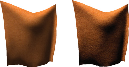
Figure 11-1 Comparing Simple Diffuse Texture Mapping and Our Method
Unfortunately, the acquisition of such material properties is fairly tedious and time-consuming (Dana et al. 1999, Lensch et al. 2001, Matusik et al. 2002). This is because material properties are specified by the four-dimensional bidirectional reflectance distribution function (BRDF), which depends on the local light and viewing directions; the Phong model is an example of a BRDF. If spatial variation across a surface is to be captured, this function (which is the bidirectional texture function we mentioned earlier [Dana et al. 1999]) becomes six-dimensional. Obviously, the acquisition of such a high-dimensional function requires taking many samples, resulting in large acquisition times (and storage requirements), which is the reason why BTF measurements are not readily available.
The benefit of capturing all this data is that BTFs generate very realistic renderings of materials, because they capture not only the local reflectance properties for each point on a surface, but also all nonlocal effects, such as self-shadowing, masking, and interreflections within a material, as seen in Figure 11-1.
Instead of acquiring a full BTF and rendering with that, we show that it is sufficient to acquire only some slices of the BTF. This allows for a simple acquisition setup (which can be done manually) and an even simpler rendering method, which runs in real time on GPUs even a few years old. An artist can also easily manipulate an acquired material, for example, making it more or less specular by manipulating a few parameters. To make this work, we assume that the captured material patch is isotropic (that is, its appearance does not depend on its orientation) and has only small-scale features (that is, no large self-shadowing and masking effects). Later on, we discuss in more detail why this is necessary.
11.2 Acquisition
The acquisition and preprocessing steps are very simple, resulting in a fast acquisition procedure.
11.2.1 Setup and Acquisition
The setup is illustrated in the top of Figure 11-2. A camera is looking orthographically at the material to be acquired. The material is assumed to be planar, so it is best to place the material patch on a flat surface. We then illuminate the surface with a parallel light source (a distant point light source works fine) at different incident elevation angles. The light source is moved only along an arc; that is, it is not rotated around the surface normal. With the light source moving along an arc, the material reveals small self-shadowing effects, which are very characteristic of many materials.
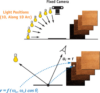
Figure 11-2 An Overview of the Capture Methodology
The light source elevation angles are (roughly) spaced in 10-degree steps; that is, we acquire ten images for every material. For real-time rendering, low-dynamic-range images work fine, as shown in Section 11.4; however, high-dynamic-range images can also be acquired.
In Figure 11-2, you can see the acquired images for a few different light source angles. We acquire all images manually, but even then the acquisition of a material takes only a few minutes, a big advantage over other methods (Dana et al. 1999, Matusik et al. 2002, Sattler et al. 2003).
11.2.2 Assembling the Shading Map
We now assemble our acquired images as a stack of images. To this end, we first compute the average radiance (or intensity) a k of each acquired image k. Because we want to index efficiently into this stack of images later on, it is useful to resample the stack so that the average radiance increases linearly. This is done by first computing what the average radiance for slice i should be, where i refers to a slice in the resampled stack:
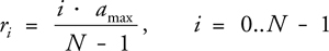
Here ri denotes the desired radiance for slice i, a max is the maximum acquired average radiance, and N is the number of slices. For each resampled slice i we now take the two original images whose average radiances ak1 and ak2 are above and below the desired radiance ri and linearly interpolate between those two images accordingly. The resulting stack of new images is called the shading map, as shown in Figure 11-3. From now on, the values stored in the shading map are interpreted as BRDF times cosine value, as explained in the next section.
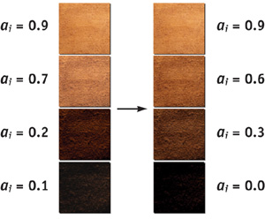
Figure 11-3 Creating a Shading Map
11.3 Rendering
As stated before, rendering with our data is fairly simple. First we give a high-level description and then go into more details.
Consider shading a fragment with an ordinary lighting model—such as the Phong model—and a point light source. In that case, we compute the amount of reflected light by evaluating the lighting model with the current view and light direction and a set of parameters such as diffuseness, specularity, and so on. This value gives us a rough idea of how bright the pixel should be. Now that we have figured out its brightness, we can use our stack of images to shade it better. We select the image in our stack that has the same average brightness as our pixel. We now look up the appropriate texel from that image and use this value instead. This will introduce the fine detail such as self-shadowing, which we have captured in our image stack, and make the rendering much more realistic.
11.3.1 Detailed Algorithm
Here we describe the computation necessary for one fragment only; obviously, it has to be repeated for every fragment. We assume that for a fragment, we are given local view and light directions (o , i ), as well as a set of texture coordinates (s, t).
First, we compute the value r by evaluating a lighting model, that is, the BRDF fr (which can be any BRDF model) multiplied by the cosine of the incident angle:

The value is used to fine-tune the shade of the material. It is needed if the acquisition is not done with a unit light source or if only low-dynamic-range images are captured.
For example, for the simple Phong model, this computation boils down to the following formula:
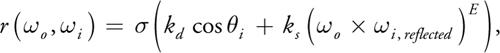
where k d and k s are the diffuse and specular coefficients, respectively, and E is the specular exponent.
Now we compute the amount of reflected light by multiplying the intensity of the incident light with the value S(r) from our shading map:
where I(i ) is the intensity of the light source (coming from i ). Using the value r(o , i ), we do a lookup into our shading map using the operator S(). It performs the lookup with the coordinates (s, t, r/a max x (N-1)), where (s, t) signifies the position in the map, and r/a max x (N - 1) is the layer to be chosen (as before, a max is the maximum acquired value and N is the number of slices). Trilinear filtering of the shading map samples should be used to avoid blockiness and contouring artifacts.
One special case needs to be treated. If the required value r is higher than the maximum average value a max in our shading map, we can either clamp the result at a max or scale the brightest image in our shading map to the desired level r i . The smallest average radiance r 0 is always zero (see Equation 1), and no special treatment is required.
11.3.2 Real-Time Rendering
The algorithm for real-time rendering using graphics hardware is straightforward. We load the shading map as a 3D (volume) texture onto the graphics hardware. In a vertex shader, we compute r( o , i ) (for a single-point light source). The result of the vertex shader is a set of texture coordinates (s, t, r/a max), which is then used to look up into the shading map. A fragment shader performs the multiplication with the intensity of the light source. See Listing 11-1 for a vertex and fragment shader performing this operation.
Newer graphics hardware supports dependent texture lookups in the fragment shaders. With this feature, it is possible to compute the BRDF (times the cosine) on a perfragment basis and then do a dependent texture lookup into the shading map, which avoids undersampling artifacts that may occur when using a vertex shader.
Example 11-1. The Vertex and Pixel Shaders Needed for Rendering
In this example, we used the enhanced Phong shading model.
// Vertex Shader
void btfv(float4 position
          : POSITION, float3 normal
          : NORMAL, float3 tex
          : TEXCOORD0, out float4 HPOS
          : POSITION, out float3 TEX
          : TEXCOORD0, out float4 COL0
          : TEXCOORD1, uniform float4x4 mvp, uniform float3 lightpos,
            uniform float3 eye, uniform float lightintensity, uniform float Ka,
            uniform float Kd, uniform float Ks, uniform float N)
{
  // compute light direction
  float3 L = lightpos - (float3)position;
  L = normalize(L);
  // compute reflected direction
  float3 R = (2.0f * dot(eye, normal) * normal - eye);
  // lighting (enhanced, physically correct Phong model)
  const float pi = 3.14159265;
  float costh = dot(normal, L);
  float specular = pow(dot(R, L), N);
  float intensity = Kd / pi + Ks * (N + 2.0) * specular / (2.0 * pi);
  intensity *= costh; // * cos(th)
  // check boundaries
  if (diffuse < 0.0 || intensity < 0.0)
    intensity = 0.0;
  if (intensity > 1.0)
    intensity = 1.0;
  // add ambient
  intensity += Ka;
  // set coordinates for lookup into volume
  TEX.z = intensity;
  // based on lighting, a_max assumed to be 1
  TEX.xy = tex.xy;
  // copy the 2D part from application
  // set light source intensity for scaling in fragment shader
  COL0.rgb = lightintensity;
  // transform position
  HPOS = mul(mvp, position);
}
// Fragment Shader
float3 btfp(float3 tc
            : TEXCOORD0, float3 color
            : TEXCOORD1, uniform sampler3D material
            : TEXUNIT0)
    : COLOR
{
  float3 r = (float3)tex3D(material, tc).xyz; // lookup into volume
  return r * color;
  // scale by intensity
}
11.4 Results
We will show several renderings with acquired materials. All materials were acquired using ten different light source positions. The images were cropped to 1024x1024 and then downscaled to 512x512. In order to be compatible with graphics hardware, which usually requires power-of-two texture sizes, we resampled these ten images down to eight images during linearization. The linearization takes about 5 seconds for each set of images. For all renderings, we have used the Phong model.
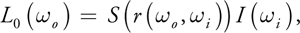
In Figure 11-4, you can see different renderings done with our real-time implementation. The materials shown are jeans (Stanford bunny and pants), suede (Stanford bunny), leather (cat), pressed wood (head), wax (head), nylon (pants), cloth (piece of cloth), and wool (piece of knit cloth).
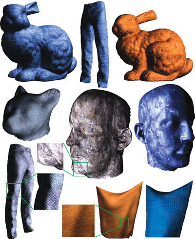
Figure 11-4 Different Models and Materials
Figure 11-5 shows a rendering of a sweater made of wool. The left image was done with a full BTF (6,500 images, compressed using principal components analysis with 16 components). The right image was done with our technique. Differences are visible mainly at grazing angles, where masking effects become important, which cannot be reproduced by our technique. This also results in slight color differences (although some color difference is also caused by the compression). Considering that wool is one of the materials that violates our initial assumptions (it has a larger-scale structure and is anisotropic), our method does fairly well.
Figure 11-5 A Sweater Made of Wool
11.4.1 Discussion
Why is it sufficient to acquire images for a fixed view and only several incident illumination directions? As stated earlier, we are acquiring only the change in illumination due to a material's surface structure, and for this purpose our method suffices. The artist supplies the actual BRDF.
We believe that this technique works so well because a human observer expects a certain kind of variation in materials. Judging from the results, this variation is captured by our technique and gives a good impression of the actual materials.
Generally speaking, materials with small-scale variations, such as the cloth, suede, jeans, and other materials shown, work best. Materials with spatially varying reflectance properties (such as different specularities, and so on) are captured well, too, as can be seen in the candle wax and pressed wood in Figure 11-4.
For certain materials, though, this technique works less well. For example, the acquisition of highly specular materials is problematic, mainly because of our use of a point light source as an approximation to a parallel light source. Our method assumes materials with a fine-scale structure. This is because our technique models variation with the incidence angle only, not with the azimuth. Therefore, shadows from larger structures cannot be captured or represented well, because they always appear in the same direction. Furthermore, the materials are assumed to be isotropic.
Even for materials violating these assumptions, our technique might still be suitable for a fast preview, because it is much better than regular texturing, as Figure 11-1 shows.
11.5 Conclusion
We have presented a method that enables acquisition and rendering of complex spatially varying materials using only a few images. This empirical method does not capture the actual BRDF but only how illumination changes due to fine surface structure; the BRDF can be adapted later. Real-time rendering using the technique can be easily implemented.
11.6 References
Dana, K., B. van Ginneken, S. Nayar, and J. Koenderink. 1999. "Reflectance and Texture of Real-World Surfaces." ACM Transactions on Graphics 18(1), January 1999, pp. 1–34.
Kautz, J., M. Sattler, R. Sarlette, R. Klein, and H.-P. Seidel. 2004. "Decoupling BRDFs from Surface Mesostructures." In Proceedings of Graphics Interface 2004, May 2004, pp. 177–184.
Lensch, H., J. Kautz, M. Goesele, W. Heidrich, and H.-P. Seidel. 2001. "Image-Based Reconstruction of Spatially Varying Materials." In 12th Eurographics Workshop on Rendering, June 2001, pp. 103–114.
Matusik, W., H. Pfister, A. Ngan, P. Beardsley, and L. McMillan. 2002. "Image-Based 3D Photography Using Opacity Hulls." ACM Transactions on Graphics (Proceedings of SIGGRAPH 2002), July 2002, pp. 427–437.
Sattler, M., R. Sarlette, and R. Klein. 2003. "Efficient and Realistic Visualization of Cloth." In Eurographics Symposium on Rendering 2003, June 2003, pp. 167–178.
Copyright
Many of the designations used by manufacturers and sellers to distinguish their products are claimed as trademarks. Where those designations appear in this book, and Addison-Wesley was aware of a trademark claim, the designations have been printed with initial capital letters or in all capitals.
The authors and publisher have taken care in the preparation of this book, but make no expressed or implied warranty of any kind and assume no responsibility for errors or omissions. No liability is assumed for incidental or consequential damages in connection with or arising out of the use of the information or programs contained herein.
NVIDIA makes no warranty or representation that the techniques described herein are free from any Intellectual Property claims. The reader assumes all risk of any such claims based on his or her use of these techniques.
The publisher offers excellent discounts on this book when ordered in quantity for bulk purchases or special sales, which may include electronic versions and/or custom covers and content particular to your business, training goals, marketing focus, and branding interests. For more information, please contact:
U.S. Corporate and Government Sales
(800) 382-3419
corpsales@pearsontechgroup.com
For sales outside of the U.S., please contact:
International Sales
international@pearsoned.com
Visit Addison-Wesley on the Web: www.awprofessional.com
Library of Congress Cataloging-in-Publication Data
GPU gems 2 : programming techniques for high-performance graphics and general-purpose
computation / edited by Matt Pharr ; Randima Fernando, series editor.
p. cm.
Includes bibliographical references and index.
ISBN 0-321-33559-7 (hardcover : alk. paper)
1. Computer graphics. 2. Real-time programming. I. Pharr, Matt. II. Fernando, Randima.
T385.G688 2005
006.66—dc22
2004030181
GeForce™ and NVIDIA Quadro® are trademarks or registered trademarks of NVIDIA Corporation.
Nalu, Timbury, and Clear Sailing images © 2004 NVIDIA Corporation.
mental images and mental ray are trademarks or registered trademarks of mental images, GmbH.
Copyright © 2005 by NVIDIA Corporation.
All rights reserved. No part of this publication may be reproduced, stored in a retrieval system, or transmitted, in any form, or by any means, electronic, mechanical, photocopying, recording, or otherwise, without the prior consent of the publisher. Printed in the United States of America. Published simultaneously in Canada.
For information on obtaining permission for use of material from this work, please submit a written request to:
Pearson Education, Inc.
Rights and Contracts Department
One Lake Street
Upper Saddle River, NJ 07458
Text printed in the United States on recycled paper at Quebecor World Taunton in Taunton, Massachusetts.
Second printing, April 2005
Dedication
To everyone striving to make today's best computer graphics look primitive tomorrow
- Copyright
- Inside Back Cover
- Inside Front Cover
- Part I: Geometric Complexity
-
- Chapter 1. Toward Photorealism in Virtual Botany
- Chapter 2. Terrain Rendering Using GPU-Based Geometry Clipmaps
- Chapter 3. Inside Geometry Instancing
- Chapter 4. Segment Buffering
- Chapter 5. Optimizing Resource Management with Multistreaming
- Chapter 6. Hardware Occlusion Queries Made Useful
- Chapter 7. Adaptive Tessellation of Subdivision Surfaces with Displacement Mapping
- Chapter 8. Per-Pixel Displacement Mapping with Distance Functions
- Part II: Shading, Lighting, and Shadows
-
- Chapter 9. Deferred Shading in S.T.A.L.K.E.R.
- Chapter 10. Real-Time Computation of Dynamic Irradiance Environment Maps
- Chapter 11. Approximate Bidirectional Texture Functions
- Chapter 12. Tile-Based Texture Mapping
- Chapter 13. Implementing the mental images Phenomena Renderer on the GPU
- Chapter 14. Dynamic Ambient Occlusion and Indirect Lighting
- Chapter 15. Blueprint Rendering and "Sketchy Drawings"
- Chapter 16. Accurate Atmospheric Scattering
- Chapter 17. Efficient Soft-Edged Shadows Using Pixel Shader Branching
- Chapter 18. Using Vertex Texture Displacement for Realistic Water Rendering
- Chapter 19. Generic Refraction Simulation
- Part III: High-Quality Rendering
-
- Chapter 20. Fast Third-Order Texture Filtering
- Chapter 21. High-Quality Antialiased Rasterization
- Chapter 22. Fast Prefiltered Lines
- Chapter 23. Hair Animation and Rendering in the Nalu Demo
- Chapter 24. Using Lookup Tables to Accelerate Color Transformations
- Chapter 25. GPU Image Processing in Apple's Motion
- Chapter 26. Implementing Improved Perlin Noise
- Chapter 27. Advanced High-Quality Filtering
- Chapter 28. Mipmap-Level Measurement
- Part IV: General-Purpose Computation on GPUS: A Primer
-
- Chapter 29. Streaming Architectures and Technology Trends
- Chapter 30. The GeForce 6 Series GPU Architecture
- Chapter 31. Mapping Computational Concepts to GPUs
- Chapter 32. Taking the Plunge into GPU Computing
- Chapter 33. Implementing Efficient Parallel Data Structures on GPUs
- Chapter 34. GPU Flow-Control Idioms
- Chapter 35. GPU Program Optimization
- Chapter 36. Stream Reduction Operations for GPGPU Applications
- Part V: Image-Oriented Computing
-
- Chapter 37. Octree Textures on the GPU
- Chapter 38. High-Quality Global Illumination Rendering Using Rasterization
- Chapter 39. Global Illumination Using Progressive Refinement Radiosity
- Chapter 40. Computer Vision on the GPU
- Chapter 41. Deferred Filtering: Rendering from Difficult Data Formats
- Chapter 42. Conservative Rasterization
- Part VI: Simulation and Numerical Algorithms
-
- Chapter 43. GPU Computing for Protein Structure Prediction
- Chapter 44. A GPU Framework for Solving Systems of Linear Equations
- Chapter 45. Options Pricing on the GPU
- Chapter 46. Improved GPU Sorting
- Chapter 47. Flow Simulation with Complex Boundaries
- Chapter 48. Medical Image Reconstruction with the FFT