
GPU Gems 2
GPU Gems 2 is now available, right here, online. You can purchase a beautifully printed version of this book, and others in the series, at a 30% discount courtesy of InformIT and Addison-Wesley.
The CD content, including demos and content, is available on the web and for download.
Chapter 44. A GPU Framework for Solving Systems of Linear Equations
Jens Krüger
Technische Universität München
Rüdiger Westermann
Technische Universität München
44.1 Overview
The development of numerical techniques for solving partial differential equations (PDEs) is a traditional subject in applied mathematics. These techniques have a variety of applications in physics-based simulation and modeling, geometry processing, and image filtering, and they have been frequently employed in computer graphics to provide realistic simulation of real-world phenomena.
One of the basic methods to solve a PDE is to transform it into a large linear system of equations via discretization. This system can then be solved using linear algebra operations.
In this chapter, we present a general framework for the computation of linear algebra operations on programmable graphics hardware. Built upon efficient representations of vectors and matrices on the GPU, vector-vector and matrix-vector operations are implemented using fragment programs on DirectX 9-class hardware. By means of these operations, implicit solvers for systems of algebraic equations can be implemented, thus enabling stable numerical simulation on programmable graphics hardware.
We describe a C++ class hierarchy that allows easy and efficient use of the proposed operations. The library provides routines for solving systems of linear equations, least-squares solutions of linear systems of equations, and standard operations on vector and matrix elements. Our system handles dense, banded, and general sparse matrices. The complete library, together with the "implicit water surface" demo (see Figure 44-9, later in the chapter), can be found on this book's CD.
We demonstrate the efficiency of our GPU solver using a particular PDE: the Poisson equation. Poisson's equation is of particular importance in physics, and its solution is frequently employed in computer graphics for the simulation of fluids and flow (as shown in Figure 44-10, later in the chapter). Throughout this chapter, we show a variety of graphics effects that involve the solution of this PDE.
44.2 Representation
To solve linear PDEs on the GPU, we need a linear algebra package. Built upon efficient GPU representations of scalar values, vectors, and matrices, such a package can implement high-performance linear algebra operations such as vector-vector and matrix-vector operations. In this section, we describe in more detail the internal representation of linear algebra operators in our GPU linear algebra library.
44.2.1 The "Single Float" Representation
In addition to representing vectors and matrices, the library needs to represent individual scalar floating-point values. At first glance, a representation of single floating-point values on the GPU might seem needless; the values could just be given via uniform program parameters. However, because many operations generate and work with single scalar values, we need to carefully choose how to represent such values on the GPU. A reasonable representation (and one that fits well with the representations of other types) is to use single-element textures. Because GPUs provide an efficient memory interface to texture data, in our system, single floating-point values are stored in textures of size 1 x 1. No matter the actual size of the GPU texture cache, we can safely assume that one float value will fit into it.
44.2.2 Vectors
Because a vector is a 1D data structure, we could simply represent a vector as a 1D texture on the GPU. The drawbacks of such a representation quickly become apparent after investigating the constraints that are imposed on textures by the GPU. All textures on current generations of GPUs are limited in size; this limit is currently 4096 for 1D textures. Thus we can represent only vectors of length 4096 using 1D textures, which is not sufficient for the simulation of reasonable problem sizes. In addition, we often will compute a vector as the result of a computation by rendering a primitive that covers the area of the vector being computed. On recent GPUs, rendering 2D textured primitives is far faster than rendering 1D primitives that generate the same number of fragments. Therefore, we reorder 1D vectors to be laid out as 2D textures on the GPU, as illustrated in Figure 44-1. To further reduce the size of the internal representation, we pack contiguous blocks of 2x2 entries into one RGBA texel. On some GPUs, this layout also improves texture access performance.
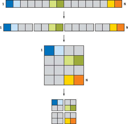
Figure 44-1 Representing a 1D Vector on the GPU
Now that we have an efficient vector representation, we can advance to a more complex linear algebra entity: the matrix.
44.2.3 Matrices
While vectors are usually treated as full vectors—vectors in which practically all elements are nonzero—matrices often have only a few nonzero entries, especially those matrices derived from PDE discretizations. Therefore, we describe different representations for different types of matrices. We start with the representation for full matrices, also called dense matrices, in which almost every value is nonzero. Later we take a look at alternative sparse matrix types.
Full Matrices
To represent a dense matrix, we split up the matrix into a set of column vectors and store each vector in the format described earlier. Figure 44-2 illustrates the procedure. As we show later, matrix-vector operations can be performed very efficiently on this representation.
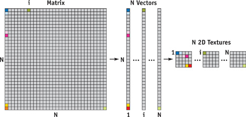
Figure 44-2 Representing a Dense Matrix on the GPU
Banded Sparse Matrices
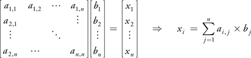
In real-world applications, sparse matrices exhibiting a regular pattern of nonzero elements often arise from domain discretizations. Banded matrices occur if computations on grid points in a regular grid involve a fixed stencil of adjacent grid points. Then, nonzero elements are arranged in a diagonal pattern. See Equation 44-1 for an example of such a matrix.
Equation 44-1 A Banded Sparse Matrix After Discretization of the 2D Wave Equation
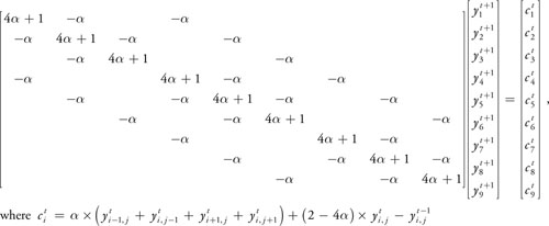
Representing such matrices as full matrices wastes a lot of space and leads to unnecessary numerical computations, because zero elements cannot easily be discarded during computations on the GPU. Therefore, we need a special representation for this type of matrix. Due to the diagonal structure, this becomes straightforward: instead of storing the columns of the matrix, we store its diagonals in the proposed vector format. Note that in this representation, some space for the off-middle diagonals is wasted and padded with zeroes. If the matrix has many nonzero diagonals and a significant amount of memory is wasted this way, we can combine two opposing diagonals into one vector. See Figure 44-3 for an example. By doing so, we can store even a full matrix in the diagonal format without wasting a single byte of texture space.
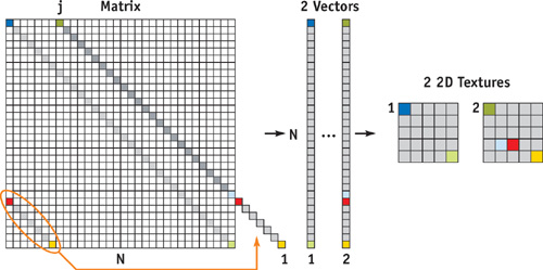
Figure 44-3 Representing a Banded Sparse Matrix on the GPU
Random Sparse Matrices
Now let's have a closer look at how to represent matrices in which nonzero elements are scattered randomly. In this case, a texture-based representation either leads to highly fragmented textures that waste a lot of space or else requires a complex indexing scheme that significantly reduces the performance of matrix access operations. For this particular kind of matrix, we prefer a vertex-based representation: We generate one vertex for sets of four nonzero entries in a matrix row. We choose the position of this vertex in such a way that it encodes the row index as a 2D coordinate; the vertex renders at exactly the same position where the respective vector element was rendered via the corresponding 2D texture. Similarly, we encode columns as 2D indices in texture coordinates 1 through 4. Matrix entries are stored in the XYZW components of the first texture coordinate of each vertex. Then we store the entire set of vertices in a vertex buffer on the GPU. As long as the matrix is not going to be modified, the internal representation does not have to be changed. The left part of Figure 44-4 shows the encoding scheme (we explain the matrix-vector product on the right side in Section 44.3.3).
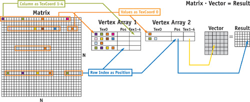
Figure 44-4 Representing a Random Sparse Matrix
44.3 Operations
Now that we have representations for scalars, vectors, and matrices, let's describe some basic operations on these representations. Again, we begin with the simplest case: a component-wise vector-vector operation.
44.3.1 Vector Arithmetic
Using the vector representation as proposed, a vector-vector operation reduces to rendering a dual-textured quad. To explain our approach, we describe the implementation of a vector-vector sum, as shown in Figure 44-5.
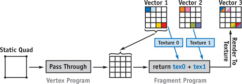
Figure 44-5 An Example of a Vector-Vector Add Operation
First we set up the viewport to cover exactly as many pixels as there are elements in the 2D target vector, and we make the target vector texture the current render target. We then render a quad that covers the entire viewport. Vertices pass through the vertex stage to the rasterizer, which generates one fragment for every vector element. For every fragment, a fragment program is executed. The program fetches respective elements from both operand vectors, adds these values together, and writes the result into the render target. Note that the result is already in the appropriate format and is ready to be used in upcoming operations. In particular, elements don't need to be rearranged, and the processing of RGBA encoded data is done simultaneously.
While the vector-vector sum operates component-wise on its input operands and outputs a vector of equal length, other operations reduce the contents of a vector to a single scalar value—for instance, computing the sum of all vector elements.
44.3.2 Vector Reduce
A vector that is represented by a texture of size nxn can be reduced to the sum of the values of its elements in log(n) passes. Starting with the original 2D texture, we set up a viewport of half the size of this texture in both directions. A full-screen quad is rendered into this viewport, and a fragment program fetches four adjacent values from the current source texture. These values are added, and they are written into the render texture target, which becomes the source texture in the next pass. We repeat this process log(n) times to produce the sum of all elements, which is written into the single float texture described earlier. Figure 44-6 gives an overview of this process.
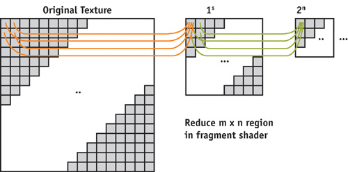
Figure 44-6 A Vector Reduction Operation
Now that we have found a way to handle component-wise operations and reduce operations, we have all we need to operate on vectors. We now advance to the matrix operations.
44.3.3 Matrix-Vector Product
The way we compute a matrix-vector product depends on whether our matrix is stored in the vector stack format (for banded and full matrices) or in the vertex format (for random sparse matrices).
Full and Banded Sparse Matrix-Vector Product
To compute a matrix-vector product, we split up the computation into a series of vector-vector products. Again, we show the process by means of an example. The banded sparse matrix-vector product and full matrix-vector product algorithms are the same. For this example, we use a matrix with two nonzero diagonals, as shown in Figure 44-7.
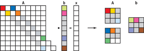
Figure 44-7 Setup for the Matrix-Vector Product · =
As we described in the previous section, the matrix A is encoded as two vectors stored in two 2D textures, and the upper diagonal is padded with zeroes. The vector is stored as a single 2D texture. We compute the final result in two passes. First we write a vector-vector product of the left diagonal and b into x. Then b is shifted by two elements and another vector-vector product of this shifted b and the second diagonal of A is added to the intermediate result of the first pass, stored in x. We perform the shift with a texture coordinate transformation, so that we don't need any expensive element moves. After these two vector-vector products, we are already done! The vector x now stores the final result of the matrix-vector product, and once again no further processing or rearranging is needed.
The only change needed to compute a full matrix-vector product is to skip the coordinate shift of b. The random sparse matrix representation, however, requires slightly different handling.
Random Sparse Matrix-Vector Product
The general approach to computing this matrix-vector product has already been encoded into the production scheme of the vertices. Let's take a look at how a result vector x is computed from a matrix A and vector b.
Equation 44-2 Matrix-Vector Product
You can see that the row index i influences the final position of the value a i, j , while the column index j specifies what values of the vector b are to be combined with a i, j . Taking a second look at Figure 44-4 reveals that for a given matrix entry, the column is encoded in the vertex position while the row is encoded as a texture coordinate. To compute the result vector x, all we have to do is render the vertices as points into the texture of x while multiplying the color values with values fetched from b using the given texture coordinates. This automatically places the values at the correct positions within the target vector and fetches the correct combination from the vector b. As always, after all points are rendered, the vector-matrix product is stored in the texture of vector x in the correct format.
Note that even though this product is computed in a completely different way compared to the full or banded sparse matrix-vector product, the input and output vector types are identical to the ones used before. This means that we can use both matrix types simultaneously in one algorithm.
44.3.4 Putting It All Together
Now that we know how to implement the very basic linear algebra operations, we can put them together into a C++ framework. Figure 44-8 shows a simplified UML diagram of how our library is organized.
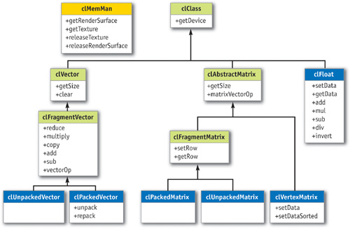
Figure 44-8 The Linear Algebra Class Collection
The classes marked in green are the interface classes; the others provide internal structure. One can see that in addition to the operations described earlier, we have implemented other methods such as data setting and getting functions—implemented as texture uploads and downloads—and packing and unpacking routines to convert from RGBA-encoded to nonencoded vectors and back. The clMemMan class is a virtual memory manager that is useful because some computations, such as reduce, need intermediate textures. Because the memory space on the GPU is limited, these textures should be shared among vectors. The clMemMan class manages a pool of textures to be used by the vectors and matrices.
44.3.5 Conjugate Gradient Solver
We now possess an easy-to-use class framework that completely abstracts the underlying hardware implementation, so we can easily write more-complex algorithms such as the conjugate gradient linear system solver. Using our implementation, the complete GPU conjugate gradient class appears in Listing 44-1.
Example 44-1. The Conjugate Gradient Solver
void clCGSolver::solveInit()
{
  Matrix->matrixVectorOp(CL_SUB, X, B, R); // R = A * x - b
  R->multiply(-1);
  // R = -R
  R->clone(P);
  // P = R
  R->reduceAdd(R, Rho);
  // rho = sum(R * R);
}
void clCGSolver::solveIteration()
{
  Matrix->matrixVectorOp(CL_NULL, P, NULL, Q);
  // Q = Ap;
  P->reduceAdd(Q, Temp);
  // temp = sum(P * Q);
  Rho->div(Temp, Alpha);
  // alpha = rho/temp;
  X->addVector(P, X, 1, Alpha);
  // X = X + alpha * P
  R->subtractVector(Q, R, 1, Alpha);
  // R = R - alpha * Q
  R->reduceAdd(R, NewRho);
  // newrho = sum(R * R);
  NewRho->divZ(Rho, Beta);
  // beta = newrho/rho
  R->addVector(P, P, 1, Beta);
  // P = R + beta * P;
  clFloat *temp;
  temp = NewRho;
  NewRho = Rho;
  Rho = temp;
  // swap rho and newrho pointers
}
void clCGSolver::solve(int maxI)
{
  solveInit();
  for (int i = 0; i < maxI; i++)
    solveIteration();
}
int clCGSolver::solve(float rhoTresh, int maxI)
{
  solveInit();
  Rho->clone(NewRho);
  for (int i = 0; i < maxI && NewRho.getData() > rhoTresh; i++)
    solveIteration();
  return i;
}
The code demonstrates the goal of our linear algebra framework: to abstract all GPU-specific details of the computation. Now, more complex algorithms can be built on top of this framework. In the following section, we demonstrate its use for numerical simulation.
44.4 A Sample Partial Differential Equation
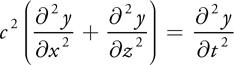
In this section, we show how to numerically solve a particular linear PDE—the 2D wave equation—on the GPU. The 2D wave equation, shown in Equation 44-3, describes the behavior of an oscillating membrane such as a shallow water surface. The equation describes the dynamic behavior of membrane displacements y depending on wave speed c. Here, t refers to time, and x and z represent the 2D spatial domain.
Equation 44-3 2D Shallow-Water Wave Equation
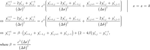
To numerically solve this PDE, we first discretize it into a set of finite-difference equations by replacing partial derivatives with central differences. A central-difference approximation can be derived from the Taylor expansion, shown in Equation 44-4. The equation shows first-order forward, backward, and central differences, as well as second-order central differences.
Equation 44-4 Taylor Expansion and Central Differences
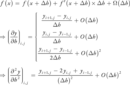
By applying the central differences of Equation 44-4 to Equation 44-3, we get the system of difference equations shown in Equation 44-5.
Equation 44-5 The Explicit Discrete 2D Wave Equation
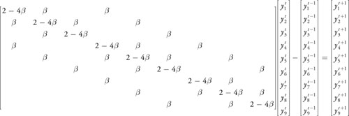
Equation 44-5 can now be rewritten as a matrix-vector operation, using the operands in Equation 44-6.
Equation 44-6 Explicit Discrete 2D Wave Equation Written as a Matrix-Vector Operation
The new values for
 can be computed easily with our framework by applying one matrix-vector operation:
clMatrix->matrixVectorOp(CL_SUB, clCurrent, clLast, clNext);
clLast->copyVector(clCurrent);
// save for next iteration
clCurrent->copyVector(clNext);
// save for next iteration
cluNext->unpack(clNext);
// unpack for rendering
renderHF(cluNext->m_pVectorTexture);
// render as height field
Although this method is very fast, it is only conditionally stable. If the integration time step becomes too large, the system will become unstable—a well-known drawback of explicit approaches. Therefore, we will employ an implicit scheme to numerically solve the wave equation.
44.4.1 The Crank-Nicholson Scheme
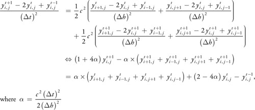
To turn this unstable discretization of the wave equation into an unconditionally stable version, we use the Crank-Nicholson scheme. In this scheme, the average of the current and the next time steps is used for the special discretization. This yields the formula shown in Equation 44-7.
Equation 44-7 Implicit Discrete 2D Wave Equation
If we write this as a matrix-vector product, we get the matrix from the beginning of this chapter in Equation
44-1. However, finding a solution for
now requires a solver for a system of linear equations. Fortunately, we have developed a solver for such
matrices already: the conjugate gradient solver. The program to implicitly solve the wave equation now looks
like this:
cluRHS->computeRHS(cluLast, cluCurrent); // generate c(i, j, t)
clRHS->repack(cluRHS);
// encode into RGBA
iSteps = pCGSolver->solve(iMaxSteps);
// solve using CG
cluLast->copyVector(cluCurrent);
// save for next iteration
clNext->unpack(cluCurrent);
// unpack for rendering
renderHF(cluCurrent->m_pVectorTexture);
As you can see, with only a few more lines of code—and with the help of the linear algebra framework—we can turn an unstable solution into an unconditionally stable version that allows us to increase the simulation step size and improve performance. Moreover, for some problems, explicit solutions do not work at all; without an implicit solver, some simulations cannot be implemented. An example is the Poisson-pressure equation that arises in the solution of the Navier-Stokes equations for fluid flow. See Figures 44-9 and 44-10.
Figure 44-9 A Navier-Stokes Fluid Dynamics Simulation
Figure 44-10 Simulation of the 2D Wave Equation on a 1024x1024 Grid
44.5 Conclusion
In this chapter, we have described a general framework for the implementation of numerical simulation techniques on graphics hardware; our emphasis has been on providing building blocks for the design of general numerical computing techniques. The framework includes our efficient internal layouts for vectors and matrices. By considering matrices as a set of diagonal or column vectors and by representing vectors as 2D texture maps, matrix-vector and vector-vector operations can be accelerated considerably compared to software-based approaches. Table 44-1 shows the performance of our framework on the NVIDIA GeForce 6800 GT, including basic framework operations and the complete sample application using the conjugate gradient solver. We achieve about the same performance on other vendors' GPUs, with some vendor-specific optimizations during initialization, such as texture allocation order.
Table 44-1. Timings for the Framework and Sample Application
|
As measured on an NVIDIA GeForce 6800 GT |
||||||
|
Resolution |
||||||
|
2048x1024 |
1024x1024 |
1024x512 |
512x512 |
512x256 |
256x256 |
|
|
Vector Reduce |
1.11 ms |
0.49 ms |
0.28 ms |
0.17 ms |
0.16 ms |
0.14 ms |
|
Vector-Vector Operation |
0.89 ms |
0.31 ms |
0.15 ms |
0.08 ms |
0.04 ms |
0.02 ms |
|
2D Wave Equation Demo |
12 fps |
27 fps |
52 fps |
102 fps |
185 fps |
335 fps |
44.6 References
Bolz, J., I. Farmer, E. Grinspun, and P. Schröder. 2003. "Sparse Matrix Solvers on the GPU: Conjugate Gradients and Multigrid." ACM Transactions on Graphics (Proceedings of SIGGRAPH 2003) 22(3), pp. 917–924.
Krüger, Jens, and Rüdiger Westermann. 2003. "Linear Algebra Operators for GPU Implementation of Numerical Algorithms." ACM Transactions on Graphics (Proceedings of SIGGRAPH 2003) 22(3), pp. 908–916.
Copyright
Many of the designations used by manufacturers and sellers to distinguish their products are claimed as trademarks. Where those designations appear in this book, and Addison-Wesley was aware of a trademark claim, the designations have been printed with initial capital letters or in all capitals.
The authors and publisher have taken care in the preparation of this book, but make no expressed or implied warranty of any kind and assume no responsibility for errors or omissions. No liability is assumed for incidental or consequential damages in connection with or arising out of the use of the information or programs contained herein.
NVIDIA makes no warranty or representation that the techniques described herein are free from any Intellectual Property claims. The reader assumes all risk of any such claims based on his or her use of these techniques.
The publisher offers excellent discounts on this book when ordered in quantity for bulk purchases or special sales, which may include electronic versions and/or custom covers and content particular to your business, training goals, marketing focus, and branding interests. For more information, please contact:
U.S. Corporate and Government Sales
(800) 382-3419
corpsales@pearsontechgroup.com
For sales outside of the U.S., please contact:
International Sales
international@pearsoned.com
Visit Addison-Wesley on the Web: www.awprofessional.com
Library of Congress Cataloging-in-Publication Data
GPU gems 2 : programming techniques for high-performance graphics and general-purpose
computation / edited by Matt Pharr ; Randima Fernando, series editor.
p. cm.
Includes bibliographical references and index.
ISBN 0-321-33559-7 (hardcover : alk. paper)
1. Computer graphics. 2. Real-time programming. I. Pharr, Matt. II. Fernando, Randima.
T385.G688 2005
006.66—dc22
2004030181
GeForce™ and NVIDIA Quadro® are trademarks or registered trademarks of NVIDIA Corporation.
Nalu, Timbury, and Clear Sailing images © 2004 NVIDIA Corporation.
mental images and mental ray are trademarks or registered trademarks of mental images, GmbH.
Copyright © 2005 by NVIDIA Corporation.
All rights reserved. No part of this publication may be reproduced, stored in a retrieval system, or transmitted, in any form, or by any means, electronic, mechanical, photocopying, recording, or otherwise, without the prior consent of the publisher. Printed in the United States of America. Published simultaneously in Canada.
For information on obtaining permission for use of material from this work, please submit a written request to:
Pearson Education, Inc.
Rights and Contracts Department
One Lake Street
Upper Saddle River, NJ 07458
Text printed in the United States on recycled paper at Quebecor World Taunton in Taunton, Massachusetts.
Second printing, April 2005
Dedication
To everyone striving to make today's best computer graphics look primitive tomorrow
- Copyright
- Inside Back Cover
- Inside Front Cover
- Part I: Geometric Complexity
-
- Chapter 1. Toward Photorealism in Virtual Botany
- Chapter 2. Terrain Rendering Using GPU-Based Geometry Clipmaps
- Chapter 3. Inside Geometry Instancing
- Chapter 4. Segment Buffering
- Chapter 5. Optimizing Resource Management with Multistreaming
- Chapter 6. Hardware Occlusion Queries Made Useful
- Chapter 7. Adaptive Tessellation of Subdivision Surfaces with Displacement Mapping
- Chapter 8. Per-Pixel Displacement Mapping with Distance Functions
- Part II: Shading, Lighting, and Shadows
-
- Chapter 9. Deferred Shading in S.T.A.L.K.E.R.
- Chapter 10. Real-Time Computation of Dynamic Irradiance Environment Maps
- Chapter 11. Approximate Bidirectional Texture Functions
- Chapter 12. Tile-Based Texture Mapping
- Chapter 13. Implementing the mental images Phenomena Renderer on the GPU
- Chapter 14. Dynamic Ambient Occlusion and Indirect Lighting
- Chapter 15. Blueprint Rendering and "Sketchy Drawings"
- Chapter 16. Accurate Atmospheric Scattering
- Chapter 17. Efficient Soft-Edged Shadows Using Pixel Shader Branching
- Chapter 18. Using Vertex Texture Displacement for Realistic Water Rendering
- Chapter 19. Generic Refraction Simulation
- Part III: High-Quality Rendering
-
- Chapter 20. Fast Third-Order Texture Filtering
- Chapter 21. High-Quality Antialiased Rasterization
- Chapter 22. Fast Prefiltered Lines
- Chapter 23. Hair Animation and Rendering in the Nalu Demo
- Chapter 24. Using Lookup Tables to Accelerate Color Transformations
- Chapter 25. GPU Image Processing in Apple's Motion
- Chapter 26. Implementing Improved Perlin Noise
- Chapter 27. Advanced High-Quality Filtering
- Chapter 28. Mipmap-Level Measurement
- Part IV: General-Purpose Computation on GPUS: A Primer
-
- Chapter 29. Streaming Architectures and Technology Trends
- Chapter 30. The GeForce 6 Series GPU Architecture
- Chapter 31. Mapping Computational Concepts to GPUs
- Chapter 32. Taking the Plunge into GPU Computing
- Chapter 33. Implementing Efficient Parallel Data Structures on GPUs
- Chapter 34. GPU Flow-Control Idioms
- Chapter 35. GPU Program Optimization
- Chapter 36. Stream Reduction Operations for GPGPU Applications
- Part V: Image-Oriented Computing
-
- Chapter 37. Octree Textures on the GPU
- Chapter 38. High-Quality Global Illumination Rendering Using Rasterization
- Chapter 39. Global Illumination Using Progressive Refinement Radiosity
- Chapter 40. Computer Vision on the GPU
- Chapter 41. Deferred Filtering: Rendering from Difficult Data Formats
- Chapter 42. Conservative Rasterization
- Part VI: Simulation and Numerical Algorithms
-
- Chapter 43. GPU Computing for Protein Structure Prediction
- Chapter 44. A GPU Framework for Solving Systems of Linear Equations
- Chapter 45. Options Pricing on the GPU
- Chapter 46. Improved GPU Sorting
- Chapter 47. Flow Simulation with Complex Boundaries
- Chapter 48. Medical Image Reconstruction with the FFT