
GPU Gems 2
GPU Gems 2 is now available, right here, online. You can purchase a beautifully printed version of this book, and others in the series, at a 30% discount courtesy of InformIT and Addison-Wesley.
The CD content, including demos and content, is available on the web and for download.
Chapter 25. GPU Image Processing in Apple's Motion
Pete Warden
Apple Computer
In this chapter I cover some of the challenges we faced, the solutions we found, and the lessons we learned while writing Motion. In here is everything we wish we had known when we started! The speed improvement over CPU-based rendering provided by pixel shaders was amazing, often ten to twenty times faster, but being on the frontier meant facing a steep hill to climb.
We needed to implement complex image-processing operations, so we needed GPUs that were able to run flexible and general-purpose pixel shaders. At the time we wrote Motion, in 2003 and early 2004, there were two families of graphics cards able to do this on the Mac: the ATI R3xx series and the NVIDIA NV34. Today newer GPUs like the NVIDIA GeForce 6 Series are available for the Apple platform. I concentrate on the R3xx and NV34 when I'm discussing implementation details, but most points may still apply to more recent hardware. The biggest differences in new hardware are much-increased resource limits, the advent of floating-point pixel support, and higher performance.
25.1 Design
GPUs are able to solve some problems much faster than CPUs can because they're highly specialized, can do many operations in parallel, and have very high speed parallel memory access. These capabilities come at a cost: GPUs trade off flexibility for speed. There are lots of problems that they just can't tackle, and it's vital to plan your application knowing their strengths and weaknesses.
25.1.1 Loves and Loathings
Some kinds of image-processing operations map well onto GPUs, and some are awkward or impossible to write in a shader. Here I describe some of these types, and how easy (or difficult) we found them to port to the GPU.
Image In, Image Out
Algorithms that take in one or more input images and output a single output image map to the GPU's capabilities in a very direct manner, giving a good chance of getting peak performance. Of course, these algorithms are very common in image processing, especially the kind needed by graphic design applications.
Image In, Statistics Out
Algorithms that take an input image and output some kind of measurement are more difficult to implement on the GPU. A good example is trying to count how many pixels in an image have different color values, creating a histogram. On the CPU this is simple: we just loop through all the image's pixels and increment an entry in an array, choosing the entry based on the color value of each pixel. In pseudocode:
 for
   <all pixels> arrayIndex = currentPixel.luminance;
 histogram[arrayIndex] += 1;
The problem with doing this in a pixel shader is that your result has to be written to a fixed location; you can't do the step where you choose which histogram entry to increment based on the pixel's luminance.
GPUs can flexibly gather inputs from many locations, based on runtime choices, but cannot as easily scatter their output to different places, based on the input data.
Almost all algorithms that output statistics or measurements need a scattering step, which makes it hard to write a good GPU implementation of them. See Chapter 32 of this book, "GPU Computation Strategies and Tips," for more information about implementing scatter algorithms on the GPU.
Color Transformations
Operations that take in a single pixel's color, apply some function to it, and output the result as a new color are great candidates for a GPU implementation. Often, simple transformations such as gamma correction or brightness adjustments can be calculated directly using a few arithmetic instructions in a pixel shader. More-involved transformations can be precalculated on the CPU and passed in as lookup tables. (See also Chapter 24, "Using Lookup Tables to Accelerate Color Transformations.")
Independent Neighborhood Operations
GPUs are well suited to reading in multiple pixels around a base position and combining them to get an output value. There may be limits on how many pixels can be combined in a single shader, but we can work around this by splitting the operation into several shaders and running multiple passes, with the intermediate results written out to OpenGL pixel buffers (pbuffers) and passed in as textures to following passes. We've had a lot of success implementing convolution filters such as edge detection and Gaussian blurring using this approach.
Sequential Neighborhood Operations
Any algorithm that needs to visit the pixels in an image in a particular order, using results from previous pixels in the same pass, won't work on a GPU. The results must be written to a texture. There's no way to tell in what order the pixels will be processed, and no way to access the result from any other pixel within the same pass. GPUs get some of their speed from doing many operations in parallel; to be able to do this, the programming model doesn't allow shaders that depend on this sort of ordering.
One example of an algorithm that doesn't translate well to the GPU is the sliding boxcar method for doing a box filter. It relies on traveling across rows and down columns, adding or subtracting from a running total to get its result at each pixel. There's no way to keep such a total in a shader, nor to ensure the rows and columns are visited in the right order.
Less obviously, per-pixel random-number generators can be tricky to implement, because they usually rely on storing a seed value that is updated every time a random value is fetched, and that seed value cannot be stored between pixels in a shader.
Conditional Execution
Any operation that contained more than a few branches had trouble fitting on a lot of the hardware we were developing on. [1] Shader support did not include any branch or jump instructions, and the only support at all for anything conditional was instructions that allowed a comparison value to decide which of two inputs gets placed into a result. This means calculating both possible results before doing the comparison, which soon requires a very long program for even a mildly complex decision tree.
25.1.2 Pick a Language
After evaluating a number of high-level GPU programming languages—including Cg, GLSL, HLSL, Direct3D's pixel shaders, and vendor-specific assembly languages—we chose to use OpenGL's low-level ARB_fragment_program extension for Motion.
The advantages of a C-like high-level language are clear: the learning curve is less steep, programs are easier to maintain, the compiler is able to apply high-level optimizations, and programs can be ported easily to different hardware.
It was still early in the evolution of the technology, however, and early versions of high-level compilers were not as mature as modern CPU compilers. Some were available on only a limited range of platforms at the time. These issues are easing as the language technology matures, but at the time of writing Motion, they were still unresolved.
The flaws of writing in an assembler-like language are equally well known: they're tough to learn, fiddly to build programs in, and tricky to debug and maintain. They do have some hidden strengths, though. Importantly for us, it was a lot easier to understand and work around the limits of specific GPUs when dealing with our shaders' low-level instructions than it would have been in a high-level language hiding those sorts of implementation details. Understanding the strengths and weaknesses of the GPUs through the instruction set also helped us to change our algorithms to improve performance.
ARB_fragment_program
We were happy with our choice of ARB_fragment_program for our shaders. We had solid support from both ATI and NVIDIA, we didn't suffer any big delays due to implementation bugs, and we learned a lot about how the GPUs worked. As expected, debugging was painful, but there were some other pleasant surprises.
The instruction set is quite elegant and orthogonal, and it mapped very well to many of the image-processing operations we were tackling. In quite a few cases, the GPU version was even easier to write than the C version! The functional style forced on us by the lack of conditional execution instructions in ARB_fragment_program also led to some unusual and fruitful approaches to porting over our CPU algorithms. Of course, more recent GPUs such as the GeForce 6 Series do support conditional execution.
25.1.3 CPU Fallback
There are going to be systems around for some time that lack GPUs capable of running the kind of shaders you need to do image processing. If you're adding GPU processing to an existing CPU-based program, then you can just disable the shaders and use the existing code on those systems. For an application built primarily for shader-capable hardware that chooses to support computers without GPUs, you need to decide how to handle running on these legacy systems.
There are two approaches to building a CPU fallback: you can write separate CPU versions of all your algorithms, or you can write a GPU emulator that will run shaders on the CPU.
Having independent CPU versions of your algorithms is extremely useful when implementing and debugging the GPU versions. We strongly recommend that you start off with this sort of reference implementation as a development aid; it's invaluable when you need to tell if a bug is a flaw in the basic algorithm or a problem in the shader implementation. The biggest drawback with this approach is the time needed to implement and maintain parallel versions of all your operations.
Writing a GPU emulator is beyond the scope of this chapter, but it's worth noting that image processing generally needs only a small subset of a GPU's features emulated, and that low-level shader languages use vector instructions that map well to the AltiVec and SSE instruction sets.
For Motion, we chose to support only GPU-capable hardware, because that included the majority of our target market of video professionals, and doing so let us concentrate our development time on expanding the application's capabilities.
25.2 Implementation
As we built Motion, we ran into a number of practical issues implementing our image-processing algorithms as shaders.
25.2.1 GPU Resource Limits
On ATI R3xx cards, the biggest difficulties were caused by the restrictions under which ARB_fragment_program shaders could actually be run. The GPU programs could have no more than 64 arithmetic and 32 texture-access instructions. The NVIDIA NV34 had a much higher limit of 1,024 total instructions. In practice, we found that ATI's instruction limits were not much of a problem for most of the operations we needed, though we had to spend time reducing the instruction count on a few of our more complex shaders.
Things were slightly complicated by instructions that mapped to multiple native assembly instructions on the GPU. For example, the SIN instruction on ATI cards executed a multiple-instruction Taylor series, rather than a single-instruction operation, as the NV34 does (which actually produces a higher-precision result than the Taylor series).
Far more serious for us was the limit of four levels of texture indirection on ATI GPUs. The ARB_fragment_program specification explains in detail what defines a level of texture indirection, but for practical purposes it limits you to a chain four-deep of dependent texture reads. A dependent texture read uses the results of a previous texture read or arithmetic instruction for its coordinates. Here's a simple example:
!!ARBfp1 .0 TEMP inputColor, tableResult;
#Read the input pixel; first level of indirection
TEX inputColor, fragment.texcoord[0], texture[0], 2D;
#Look up a result from a table; second level of indirection
TEX tableResult, inputColor, texture[1], 3D;
#Look up the output in a palette texture; third level of indirection
TEX result.color, tableResult, texture[2], 1D;
END
This is an example of a typical operation we'd want to do, and it's already just one level away from the limit.
Avoiding texture indirections became a major headache as we wrote our shaders. One useful approach was moving as many calculations as possible to the vertex level, because reads using interpolated vertex components or program constants do not trigger an indirection. Because we hit the indirection limit more often than we ran out of instructions, we got into the habit of burning up arithmetic instructions to do calculations on the fly rather than reading them from precalculated tables stored in textures. As a last resort, we also broke up algorithms into multiple passes, passing intermediate results between the shader stages in pbuffers. We preferred to avoid this, though, as the pbuffers available on our platform were normally 8-bit-per-channel rather than the internal shader precision of an IEEE 32-bit float on NVIDIA GPUs, or 24-bit floating point on ATI GPUs. Running multiple passes also meant a performance loss.
25.2.2 Division by Zero
The NV34 has generous instruction limits, and no cap on levels of texture indirection, but its handling of divisions by zero forced us to rewrite some of our shaders.
When an R3xx hits an RCP or RSQ instruction with an input of zero, it sets the result to be a very large number. The NV34 correctly follows the IEEE floating-point standard in these situations and outputs a "not a number" (NaN) value, representing either positive or negative infinity, depending on the sign of the numerator. The big difference between this NaN and ATI's big number is that the NaN causes the result of any math instruction it's used in to also become a NaN.
In our specific shaders, we could actually capitalize on the non-IEEE-compliant behavior, because where we had divisions by zero, they were followed by later multiplications by zero. A common example was taking a premultiplied color input, dividing the color channels by alpha to do some calculations in straight color space, and then multiplying by that same input alpha to put the result back in premultiplied space. On an R3xx, when the alpha value was zero, the output red, green, and blue channels would also be zero, which is what we desired. A NaN, however, would propagate to the output, where it would be stored as pure white in the frame buffer, which was undesirable to say the least.
Our solution was to ensure that those instructions never get passed a denominator of zero, at the cost of a few extra instructions. The general idea was to nudge the denominator a very small amount away from zero, by adding a small epsilon value if it was positive:
CMP epsilonFudge, denominator.x, 0, 0.00001;
ADD denominator.x, denominator.x, epsilonFudge;
RCP reciprocal.x, denominator.x;
This adds two extra instructions per division, but if you know the denominator will never be negative—for example, when it's been read from an 8-bit texture—you can skip the comparison like this:
ADD denominator.x, denominator.x, 0.00001;
RCP reciprocal.x, denominator.x;
Though this may look as if it sacrifices precision, the epsilon value is so small that in practice it gets lost in the underflow when added to anything but numbers very close to zero.
25.2.3 Loss of Vertex Components
As we mentioned earlier, it can be very useful to pass in vertex components interpolated across a quad into a fragment program. There are eight sets of texture coordinates available to shaders in OpenGL, but we found we could access only the first four of these on some GPUs when using OpenGL's "old-style" fixed-function vertex pipeline. Inserting a simple vertex program that simply passed through all eight coordinates solved the problem.
25.2.4 Bilinear Filtering
The basic way to do image processing using a graphics card is to draw a screen-aligned quad with the image texture mapped onto it, into a frame buffer that will hold the output image. For our compositing package, we often wanted to apply simple geometric transformations to our images, moving, scaling, or rotating them. This is easy to do on a GPU: you just need to transform a quad's vertices and pass them on to the rasterizer. These transforms can be combined with other operations implemented in fragment programs, for no extra cost. To get decent output quality, we used bilinear filtering on the input image, which also comes for free. Because bilinear filtering was so useful and had no performance cost, we used it everywhere by default. This led to two of our trickiest problems: softening and alpha fringes.
Softening
We noticed a subtle blurring or softening of images that we were drawing with no transformations—a problem that got worse as an image went through more stages of the render pipeline. We spent some time making sure that we were setting up our vertex positions and texture coordinates correctly, but it turned out to be caused by a precision problem in the way that graphics hardware rasterizes primitives. Figure 25-1 illustrates the situation.
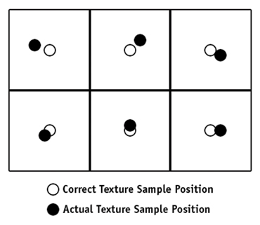
Figure 25-1 Texture Sample Position
The texture coordinates for each pixel inside a quad are calculated based on that pixel's distance from each vertex and the texture coordinates that have been set at each vertex. Because this calculation is done for each pixel drawn, everything possible is done to speed it up. Unfortunately for us, some of the optimizations used in graphics hardware trade accuracy for speed in ways that affect us a lot more than they do 3D scene rendering. When rendering scenes, all primitives will be transformed and distorted anyway, so precision errors in texture mapping that are much less than a pixel in size will not be noticeable, as long as the errors are consistent.
But we were trying to draw quads where all the pixels in the input texture were drawn into exactly the same position in the output buffer. Errors of even a fraction of a pixel away from a texel center made the bilinear filtering bleed parts of neighboring pixels into the result, causing the softening we were seeing. The amount of error depended on the way that a specific GPU implemented its texture coordinate calculations (for example, we saw much smaller errors on the NV34 than on ATI GPUs, because the NV34 has many more bits of subpixel precision). See Figure 25-2.
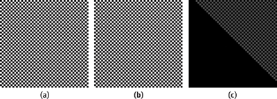
Figure 25-2 A 2x2-Pixel Checkerboard Pattern
We solved this problem in most cases by switching to nearest-neighborhood filtering where we knew we wanted one-to-one mapping. Because the errors were much less than 1 pixel wide, this produced the result we were after. The errors seemed to grow with the size of the quad, so one method we worked on was splitting a large quad into a grid of much smaller quads, doing the texture coordinate interpolation precisely on the CPU, and then storing the values into the vertices of this grid. This approach greatly reduced the error.
Alpha Fringes
The other bilinear filtering problem we hit was the dark fringes we were seeing around the alpha edges of our rendered objects, wherever any transformation caused the filtering to kick in. See Figure 25-3 for an example.
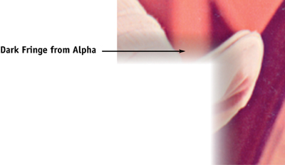
Figure 25-3 Fringing Using Bilinear Filtering
Our pipeline was based on rendering to and from pbuffer textures stored in the non-premultiplied alpha format, and this turned out to be the root of our problem. To see what was happening, look at the white, fully opaque pixel surrounded by a sea of completely transparent pixels in Figure 25-4. (Because the transparent pixels have zero alpha values and this is a straight alpha texture, it shouldn't matter what we put in their color channels, so I've set them up as black.)
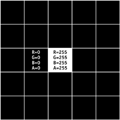
Figure 25-4 A White, Fully Opaque Pixel Surrounded by Transparent Pixels
Bilinear filtering works by taking the four closest pixels and calculating a result by mixing them together in different proportions. Figure 25-5\ shows the values you get when you draw this texture scaled up by a factor of three using bilinear filtering, and Figure 25-6 shows what happens when you composite Figure 25-5 on top of another image using the Over operator.
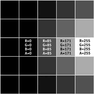
Figure 25-5 A Portion of the Result After Scaling Up the Texture Three Times with Bilinear Filtering
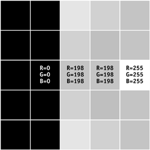
Figure 25-6 Compositing with the Over Operator
Bilinear interpolation deals with all channels separately and mixes in the color of a fully transparent pixel anywhere there's a fully or partially opaque pixel with a zero-alpha neighbor. In our case, this resulted in a gray fringe when it was blended, because the black was mixed in from the fully transparent pixels.
The usual solution to this is to ensure that zero-alpha pixels with opaque neighbors have sensible values in their color channels. This works well in a 3D-modeling context: content creators can manually fix their textures to fit within this constraint, or the textures can be run through an automated process to set sensible values, as part of the normal texture-loading pipeline.
When we're doing image processing for compositing, though, texture creation is a much more dynamic process; there's no way to intervene manually, and running a fix-up pass on each intermediate texture would be a big hit on performance. One alternative we considered was hand-rolling our own bilinear filtering in a pixel shader and discarding the influence of any fully transparent pixels. This would mean replacing every texture read with four reads wherever we wanted to use bilinear filtering, and extra arithmetic instructions to do the filtering. We ruled out this approach as impractical.
Our eventual solution was to switch our pipeline over to using textures stored in the premultiplied alpha, or associated alpha, format. Bilinear filtering using premultiplied colors doesn't suffer from the fringing problem. See Figure 25-7.
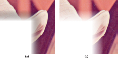
Figure 25-7 Using Premultiplied Format to Eliminate Dark Fringing
This is also the format that colors need to be in when calculating blurs, though most color-correction operations need to happen in straight-alpha color space. This pipeline change was disruptive because it happened late in development, but once everything had settled down, it worked well for us. Converting between the two color spaces in our shaders when we needed to wasn't difficult, though the division-by-zero differences discussed earlier did complicate things.
25.2.5 High-Precision Storage
Motion uses mostly 8-bit-per-channel images in its pipeline, but there were some places where more precision was needed. We implemented motion blur using an accumulation buffer algorithm, and the banding was unacceptable when using an 8-bit buffer.
At the time of writing, R3xx GPUs supported 16- and 32-bit-per-channel floating-point formats, so all we needed to do was request and create a 16-bit pbuffer. It was surprisingly easy to switch over our render pipeline to run at higher precisions; doing the same in a CPU image-processing pipeline is a lot more work. There are some restrictions on blending and filtering with high-precision pbuffers, but we were able to double-buffer two pbuffers to emulate the additive blending needed for motion blur. [2]
At the time we wrote Motion, the NV34 Mac drivers exposed support for only 8-bit-per-channel textures, so we needed an alternative implementation of motion blur that didn't use the floating-point formats. The flexibility of pixel shaders came in handy, as it enabled us to emulate a 16-bit-per-channel fixed-point pbuffer using two 8-bit textures. The accumulation buffer needed to sum up to 256 8-bit samples, so we chose to use an 8.8 fixed-point format, packing the whole number and fractional parts of each color channel into an 8-bit channel in the pbuffer, so that each color channel needed two channels in the stored texture.
Packing the value into two channels meant dividing the original value by 256, to get the whole-number part into a range where it wouldn't get clipped, and taking the modulo of the value with 1, to get the fractional part to store:
MUL output.x, value.x, reciprocalOf256;
FRC output.y, value.x;
Reconstructing the packed value meant multiplying the whole-number part stored in one channel by 256 and adding it to the fractional part to get the original value.
MAD value.x, input.x, 256, input.y;Implementing the accumulation buffer algorithm took two shader passes: one dealing with the red and green channels, the other with the blue and alpha, because a shader then could output its results to only one buffer at a time, and each buffer could hold only two channels.
25.3 Debugging
We spent a lot of time trying to figure out why our shaders weren't working. There are some debugging tools that work with ARB_fragment_program shaders—notably Apple's Shader Builder and the open source ShaderSmith project—but there was nothing available that would let us debug our GPU programs as they ran within our application. We had to fall back to some old-fashioned techniques to pry open the black box of the GPU.
Syntax errors were easiest to track down: invalid programs give a white output when they're used, just like using invalid textures. When you first load a program, calling glGetString(GL_PROGRAM_ERROR_STRING) will return a message describing any syntax error that was found.
In theory, detecting when a program has too many instructions or levels of texture indirection should just need the following call:
glGetProgramivARB(GL_fragment_program_ARB, GL_PROGRAM_UNDER_NATIVE_LIMITS_ARB,
                  &isUnderNativeLimits)
In practice, this didn't always detect when such a limit was hit, and we learned to recognize the completely black output we'd get when we went over limits on ATI GPUs. We found that the best way to confirm we had a limit problem and not a calculation error was to put a MOV result.color, { 1, 1, 0, 1 } instruction at the end of the shader. If the output became yellow, then the shader was actually executing, but if it remained black, then the program was not executing because it was over the GPU's limits.
To understand what limit we were hitting, we could comment out instructions and run the program again. Eventually, after we cut enough instructions, we'd see yellow. The type of instructions that were cut last would tell us which limit we had hit.
The nastiest errors to track down were mistakes in our logic or math, because we really needed to see the inner workings of the shader while it was running to understand what was going wrong. We found that the best way to start debugging this sort of problem was to have a simple CPU version of the algorithm that we knew was working; then we would step through the shader instruction by instruction, comparing by eye each instruction with that of the equivalent stage in the CPU implementation.
When this sort of inspection doesn't work, there's only one way to get information out of a shader: by writing it to the frame buffer. First you need to comment out the final output instruction and, instead, store some intermediate value you're interested in. You may need to scale this value so that it's in the 0–1 range storable in a normal buffer. You can then use glReadPixels() to retrieve the exact values, but often the rough color shown on screen is enough to help figure out what's happening.
If something's really baffling, try it on different GPUs, to make sure that the problem isn't caused by differences in the vendors' implementations.
25.4 Conclusion
Trying to use hardware designed for games to do high-quality image processing was both frustrating and rewarding for us. The speed of the GPU didn't just help us to convert existing algorithms; it also inspired us to experiment with new ideas. The ability to see our results instantly, combined with the convenience of reloading shaders while the application was running, gave us a fantastic laboratory in which to play with images.
25.5 References
ARB_fragment_program Specification. Not light reading, but Table X.5 has a good summary of all instructions, and Section 3.11.5 has full explanations of how each one works. http://oss.sgi.com/projects/ogl-sample/registry/ARB/fragment_program.txt
Apple's OpenGL Web Site. Lots of developer information and some great tools. http://developer.apple.com/graphicsimaging/opengl/
GPGPU Web Site. News and links to current research and tools. http://www.gpgpu.org/
My thanks to the Apple OpenGL and Core Imaging teams; to ATI and NVIDIA for making all this possible; to all the Motion team; and in particular to Tim Connolly and Richard Salvador, who generously shared their expertise.
Copyright
Many of the designations used by manufacturers and sellers to distinguish their products are claimed as trademarks. Where those designations appear in this book, and Addison-Wesley was aware of a trademark claim, the designations have been printed with initial capital letters or in all capitals.
The authors and publisher have taken care in the preparation of this book, but make no expressed or implied warranty of any kind and assume no responsibility for errors or omissions. No liability is assumed for incidental or consequential damages in connection with or arising out of the use of the information or programs contained herein.
NVIDIA makes no warranty or representation that the techniques described herein are free from any Intellectual Property claims. The reader assumes all risk of any such claims based on his or her use of these techniques.
The publisher offers excellent discounts on this book when ordered in quantity for bulk purchases or special sales, which may include electronic versions and/or custom covers and content particular to your business, training goals, marketing focus, and branding interests. For more information, please contact:
U.S. Corporate and Government Sales
(800) 382-3419
corpsales@pearsontechgroup.com
For sales outside of the U.S., please contact:
International Sales
international@pearsoned.com
Visit Addison-Wesley on the Web: www.awprofessional.com
Library of Congress Cataloging-in-Publication Data
GPU gems 2 : programming techniques for high-performance graphics and general-purpose
computation / edited by Matt Pharr ; Randima Fernando, series editor.
p. cm.
Includes bibliographical references and index.
ISBN 0-321-33559-7 (hardcover : alk. paper)
1. Computer graphics. 2. Real-time programming. I. Pharr, Matt. II. Fernando, Randima.
T385.G688 2005
006.66—dc22
2004030181
GeForce™ and NVIDIA Quadro® are trademarks or registered trademarks of NVIDIA Corporation.
Nalu, Timbury, and Clear Sailing images © 2004 NVIDIA Corporation.
mental images and mental ray are trademarks or registered trademarks of mental images, GmbH.
Copyright © 2005 by NVIDIA Corporation.
All rights reserved. No part of this publication may be reproduced, stored in a retrieval system, or transmitted, in any form, or by any means, electronic, mechanical, photocopying, recording, or otherwise, without the prior consent of the publisher. Printed in the United States of America. Published simultaneously in Canada.
For information on obtaining permission for use of material from this work, please submit a written request to:
Pearson Education, Inc.
Rights and Contracts Department
One Lake Street
Upper Saddle River, NJ 07458
Text printed in the United States on recycled paper at Quebecor World Taunton in Taunton, Massachusetts.
Second printing, April 2005
Dedication
To everyone striving to make today's best computer graphics look primitive tomorrow
- Copyright
- Inside Back Cover
- Inside Front Cover
- Part I: Geometric Complexity
-
- Chapter 1. Toward Photorealism in Virtual Botany
- Chapter 2. Terrain Rendering Using GPU-Based Geometry Clipmaps
- Chapter 3. Inside Geometry Instancing
- Chapter 4. Segment Buffering
- Chapter 5. Optimizing Resource Management with Multistreaming
- Chapter 6. Hardware Occlusion Queries Made Useful
- Chapter 7. Adaptive Tessellation of Subdivision Surfaces with Displacement Mapping
- Chapter 8. Per-Pixel Displacement Mapping with Distance Functions
- Part II: Shading, Lighting, and Shadows
-
- Chapter 9. Deferred Shading in S.T.A.L.K.E.R.
- Chapter 10. Real-Time Computation of Dynamic Irradiance Environment Maps
- Chapter 11. Approximate Bidirectional Texture Functions
- Chapter 12. Tile-Based Texture Mapping
- Chapter 13. Implementing the mental images Phenomena Renderer on the GPU
- Chapter 14. Dynamic Ambient Occlusion and Indirect Lighting
- Chapter 15. Blueprint Rendering and "Sketchy Drawings"
- Chapter 16. Accurate Atmospheric Scattering
- Chapter 17. Efficient Soft-Edged Shadows Using Pixel Shader Branching
- Chapter 18. Using Vertex Texture Displacement for Realistic Water Rendering
- Chapter 19. Generic Refraction Simulation
- Part III: High-Quality Rendering
-
- Chapter 20. Fast Third-Order Texture Filtering
- Chapter 21. High-Quality Antialiased Rasterization
- Chapter 22. Fast Prefiltered Lines
- Chapter 23. Hair Animation and Rendering in the Nalu Demo
- Chapter 24. Using Lookup Tables to Accelerate Color Transformations
- Chapter 25. GPU Image Processing in Apple's Motion
- Chapter 26. Implementing Improved Perlin Noise
- Chapter 27. Advanced High-Quality Filtering
- Chapter 28. Mipmap-Level Measurement
- Part IV: General-Purpose Computation on GPUS: A Primer
-
- Chapter 29. Streaming Architectures and Technology Trends
- Chapter 30. The GeForce 6 Series GPU Architecture
- Chapter 31. Mapping Computational Concepts to GPUs
- Chapter 32. Taking the Plunge into GPU Computing
- Chapter 33. Implementing Efficient Parallel Data Structures on GPUs
- Chapter 34. GPU Flow-Control Idioms
- Chapter 35. GPU Program Optimization
- Chapter 36. Stream Reduction Operations for GPGPU Applications
- Part V: Image-Oriented Computing
-
- Chapter 37. Octree Textures on the GPU
- Chapter 38. High-Quality Global Illumination Rendering Using Rasterization
- Chapter 39. Global Illumination Using Progressive Refinement Radiosity
- Chapter 40. Computer Vision on the GPU
- Chapter 41. Deferred Filtering: Rendering from Difficult Data Formats
- Chapter 42. Conservative Rasterization
- Part VI: Simulation and Numerical Algorithms
-
- Chapter 43. GPU Computing for Protein Structure Prediction
- Chapter 44. A GPU Framework for Solving Systems of Linear Equations
- Chapter 45. Options Pricing on the GPU
- Chapter 46. Improved GPU Sorting
- Chapter 47. Flow Simulation with Complex Boundaries
- Chapter 48. Medical Image Reconstruction with the FFT