
GPU Gems 2
GPU Gems 2 is now available, right here, online. You can purchase a beautifully printed version of this book, and others in the series, at a 30% discount courtesy of InformIT and Addison-Wesley.
The CD content, including demos and content, is available on the web and for download.
Chapter 16. Accurate Atmospheric Scattering
Sean O'Neil
16.1 Introduction
Generating realistic atmospheric scattering for computer graphics has always been a difficult problem, but it is very important for rendering realistic outdoor environments. The equations that describe atmospheric scattering are so complex that entire books have been dedicated to the subject. Computer graphics models generally use simplified equations, and very few of them run at interactive frame rates. This chapter explains how to implement a real-time atmospheric scattering algorithm entirely on the GPU using the methods described in Nishita et al. 1993. Figure 16-1 shows screenshots from the scattering demo included on this book's CD.
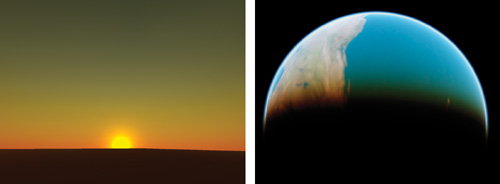
Figure 16-1 Screenshots from the Scattering Demo
Many atmospheric scattering models assume that the camera is always on or very close to the ground. This makes it easier to assume that the atmosphere has a constant density at all altitudes, which simplifies the scattering equations in Nishita et al. 1993 tremendously. Refer to Hoffman and Preetham 2002 for an explanation of how to implement these simplified equations in a GPU shader. This implementation produces an attractive scattering effect that is very fast on DirectX 8.0 shaders. Unfortunately, it doesn't always produce very accurate results, and it doesn't work well for a flight or space simulator, in which the camera can be located in space or very high above the ground.
This chapter explains how to implement the full equations from Nishita et al. 1993 in a GPU shader that runs at interactive frame rates. These equations model the atmosphere more accurately, with density falling off exponentially as altitude increases. O'Neil 2004 describes a similar algorithm that ran on the CPU, but that algorithm was too CPU-intensive. It was based on a precalculated 2D lookup table with four floating-point channels. Calculating the color for each vertex required several lookups into the table, with extra calculations around each lookup. At the time that article was written, no GPU could support such operations in a shader in one pass.
In this chapter, we eliminate the lookup table without sacrificing image quality, allowing us to implement the entire algorithm in a GPU shader. These shaders are small and fast enough to run in real time on most GPUs that support DirectX Shader Model 2.0.
16.2 Solving the Scattering Equations
The scattering equations have nested integrals that are impossible to solve analytically; fortunately, it's easy to numerically compute the value of an integral with techniques such as the trapezoid rule. Approximating an integral in this manner boils down to a weighted sum calculated in a loop. Imagine a line segment on a graph: break up the segment into n sample segments and evaluate the integrand at the center point of each sample segment. Multiply each result by the length of the sample segment and add them all up. Taking more samples makes the result more accurate, but it also makes the integral more expensive to calculate.
In our case, the line segment is a ray from the camera through the atmosphere to a vertex. This vertex can be part of the terrain, part of the sky dome, part of a cloud, or even part of an object in space such as the moon. If the ray passes through the atmosphere to get to the vertex, scattering needs to be calculated. Every ray should have two points defined that mark where the ray starts passing through the atmosphere and where it stops passing through the atmosphere. We'll call these points A and B, and they are shown in Figure 16-2. When the camera is inside the atmosphere, A is the camera's position. When the vertex is inside the atmosphere, B is the vertex's position. When either point is in space, we perform a sphere-intersection check to find out where the ray intersects the outer atmosphere, and then we make the intersection point A or B.
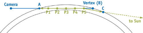
Figure 16-2 The Geometry of Atmospheric Scattering
Now we have a line segment defined from point A to point B, and we want to approximate the integral that describes the atmospheric scattering across its length. For now let's take five sample positions and name their points P 1 through P 5. Each point P 1 through P 5 represents a point in the atmosphere at which light scatters; light comes into the atmosphere from the sun, scatters at that point, and is reflected toward the camera. Consider the point P 5, for example. Sunlight goes directly from the sun to P 5 in a straight line. Along that line the atmosphere scatters some of the light away from P 5. At P 5, some of this light is scattered directly toward the camera. As the light from P 5 travels to the camera, some of it gets scattered away again.
16.2.1 Rayleigh Scattering vs. Mie Scattering
Another important detail is related to how the light scattering at the point P is modeled. Different particles in the atmosphere scatter light in different ways. The two most common forms of scattering in the atmosphere are Rayleigh scattering and Mie scattering. Rayleigh scattering is caused by small molecules in the air, and it scatters light more heavily at the shorter wavelengths (blue first, then green, and then red). The sky is blue because the blue light bounces all over the place, and ultimately reaches your eyes from every direction. The sun's light turns yellow/orange/red at sunset because as light travels far through the atmosphere, almost all of the blue and much of the green light is scattered away before it reaches you, leaving just the reddish colors.
Mie scattering is caused by larger particles in the air called aerosols (such as dust and pollution), and it tends to scatter all wavelengths of light equally. On a hazy day, Mie scattering causes the sky to look a bit gray and causes the sun to have a large white halo around it. Mie scattering can also be used to simulate light scattered from small particles of water and ice in the air, to produce effects like rainbows, but that is beyond the scope of this chapter. (Refer to Brewer 2004 for more information.)
16.2.2 The Phase Function
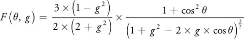
The phase function describes how much light is scattered toward the direction of the camera based on the angle (the angle between the two green rays in Figure 16-2) and a constant g that affects the symmetry of the scattering. There are many different versions of the phase function. This one is an adaptation of the Henyey-Greenstein function used in Nishita et al. 1993.
Rayleigh scattering can be approximated by setting g to 0, which greatly simplifies the equation and makes it symmetrical for positive and negative angles. Negative values of g scatter more light in a forward direction, and positive values of g scatter more light back toward the light source. For Mie aerosol scattering, g is usually set between -0.75 and -0.999. Never set g to 1 or -1, as it makes the equation reduce to 0.
16.2.3 The Out-Scattering Equation
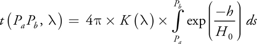
The out-scattering equation is the inner integral mentioned earlier. The integral part determines the "optical depth," or the average atmospheric density across the ray from point Pa to point Pb multiplied by the length of the ray. This is also called the "optical length" or "optical thickness." Think of it as a weighting factor based on how many air particles are in the path of the light along the ray. The rest of the equation is made up of constants, and they determine how much of the light those particles scatter away from the ray.
To compute the value of this integral, the ray from Pa to Pb will be broken up into segments and the exponential term will be evaluated at each sample point. The variable h is the height of the sample point. In my implementation, the height is scaled so that 0 represents sea level and 1 is at the top of the atmosphere. In theory, the atmosphere has no fixed top, but for practical purposes, we have to choose some height at which to render the sky dome. H 0 is the scale height, which is the height at which the atmosphere's average density is found. My implementation uses 0.25, so the average density is found 25 percent of the way up from the ground to the sky dome.
The constant is the wavelength (or color) of light and K() is the scattering constant, which is dependent on the density of the atmosphere at sea level. Rayleigh and Mie scattering each have their own scattering constants, including the scale height (H 0). Rayleigh and Mie scattering also differ in how they depend on wavelength. The Rayleigh scattering constant is usually divided by 4. In most computer graphics models, the Mie scattering constant is not dependent on wavelength, but at least one implementation divides it by 0.84. Wherever this equation depends on wavelength, it must be solved separately for each of the three color channels and separately for each type of scattering.
16.2.4 The In-Scattering Equation

The in-scattering equation describes how much light is added to a ray through the atmosphere due to light scattering from the sun. For each point P along the ray from Pa to Pb , PPc is the ray from the point to the sun and PPa is the ray from the sample point to the camera. The out-scattering function determines how much light is scattered away along the two green rays in Figure 16-2. The remaining light is scaled by the phase function, the scattering constant, and the intensity of the sunlight, Is (). The sunlight intensity does not have to be dependent on wavelength, but this is where you would apply the color if you wanted to create an alien world revolving around a purple star.
16.2.5 The Surface-Scattering Equation
|
I'v () = Iv () + I e() x exp (–t (Pa Pb , )) |
To scatter light reflected from a surface, such as the surface of a planet, you must take into account the fact that some of the reflected light will be scattered away on its way to the camera. In addition, extra light is scattered in from the atmosphere. Ie () is the amount of light emitted or reflected from a surface, and it is attenuated by an out-scattering factor. The sky is not a surface that can reflect or emit light, so only Iv () is needed to render the sky. Determining how much light is reflected or emitted by a surface is application-specific, but for reflected sunlight, you need to account for the out-scattering that takes place before the sunlight strikes the surface (that is, Is () x exp(-t(Pc Pb ,))), and use that as the color of the light when determining how much light the surface reflects.
16.3 Making It Real-Time
Let's find out how poorly these equations will perform if they're implemented as explained in the preceding section, with five sample points for the in-scattering equation and five sample points for each of the integrals to compute the out-scattering equations. This gives 5 x (5 + 5) samples at which to evaluate the functions for each vertex. We also have two types of scattering, Rayleigh and Mie, and we have to calculate each one for the different wavelengths of each of the three color channels (RGB). So now we're up to approximately 2 x 3 x 5 x (5 + 5), or 300 computations per vertex. To make matters worse, the visual quality suffers noticeably when using only five samples for each integral. O'Neil 2004 used 50 samples for the inner integrals and five for the outer integral, which pushes the number of calculations up to 3,000 per vertex!
We don't need to go any further to know that this will not run very fast. Nishita et al. 1993 used a precalculated 2D lookup table to cut the number of calculations in half, but it still won't run in real time. Their lookup table took advantage of the fact that the sun is so far away that its rays can be considered parallel. (This idea is reflected in the in-scattering equation, in Section 16.2.4.) This makes it possible to calculate a lookup table that contains the amount of out-scattering for rays going from the sun to any point in the atmosphere. This table replaces one of the out-scattering integrals with a lookup table whose variables are altitude and angle to the sun. Because the rays to the camera are not parallel, the out-scattering integral for camera rays still had to be solved at runtime.
In O'Neil 2004, I proposed a better 2D lookup table that allows us to avoid both out-scattering integrals. The first dimension, x, takes a sample point at a specific altitude above the planet, with 0.0 being on the ground and 1.0 being at the top of the atmosphere. The second dimension, y, represents a vertical angle, with 0.0 being straight up and 1.0 being straight down. At each (x, y) pair in the table, a ray is fired from a point at altitude x to the top of the atmosphere along angle y. The lookup table had four channels, two reserved for Rayleigh scattering and two reserved for Mie scattering. One channel for each simply contained the atmospheric density at that altitude, or exp(-h/H 0). The other channel contained the optical depth of the ray just described. Because the lookup table was precomputed, I chose to use 50 samples to approximate the optical depth integral, resulting in very good accuracy.
As with the lookup table proposed in Nishita et al. 1993, we can get the optical depth for the ray to the sun from any sample point in the atmosphere. All we need is the height of the sample point (x) and the angle from vertical to the sun (y), and we look up (x, y) in the table. This eliminates the need to calculate one of the out-scattering integrals. In addition, the optical depth for the ray to the camera can be figured out in the same way, right? Well, almost. It works the same way when the camera is in space, but not when the camera is in the atmosphere. That's because the sample rays used in the lookup table go from some point at height x all the way to the top of the atmosphere. They don't stop at some point in the middle of the atmosphere, as they would need to when the camera is inside the atmosphere.
Fortunately, the solution to this is very simple. First we do a lookup from sample point P to the camera to get the optical depth of the ray passing through the camera to the top of the atmosphere. Then we do a second lookup for the same ray, but starting at the camera instead of starting at P. This will give us the optical depth for the part of the ray that we don't want, and we can subtract it from the result of the first lookup. Examine the rays starting from the ground vertex (B 1) in Figure 16-3 for a graphical representation of this.
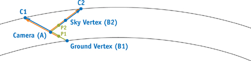
Figure 16-3Problems with the Improved Lookup Table
There's only one problem left. When a vertex is above the camera in the atmosphere, the ray from sample point P through the camera can pass through the planet itself. The height variable is not expected to go so far negative, and it can cause the numbers in the lookup table to go extremely high, losing precision and sometimes even encountering a floating-point overflow. The way to avoid this problem is to reverse the direction of the rays when the vertex is above the camera. Examine the rays passing through the sky vertex (B 2) in Figure 16-3 for a graphical representation of this.
So now we've reduced 3,000 calculations per vertex to something closer to 2 x 3 x 5 x (1 + 1), or 60 (assuming five samples for the out-scattering integral for the eye ray). Implemented in software on an Athlon 2500+ with an inefficient brute-force rendering method, I was able to get this method to run between 50 and 100 frames per second.
16.4 Squeezing It into a Shader
At this point, I felt that this algorithm had been squeezed about as much as it could, but I knew that I had to squeeze it even smaller to fit it into a shader. I didn't want this algorithm to require Shader Model 3.0, so having lookup tables in textures used by the vertex shaders wasn't possible. I decided to take a different approach and started to mathematically analyze the results of the lookup table. Even though I knew I couldn't come up with a way to simplify the integral equations, I had hoped that I might be able to simulate the results closely enough with a completely different equation.
16.4.1 Eliminating One Dimension
I started by plotting the results of the lookup table on a graph. I plotted height from 0.0 to 1.0 along the x axis and the lookup table result (optical depth) along the y axis. For various angles sampled from 0 to 1, I plotted a separate line on the graph. I noticed right away that each line dropped off exponentially as x went from 0 to 1, but the scale of each line on the graph varied dramatically. This makes sense, because as the angle of the ray goes from straight up to straight down, the length of the ray increases dramatically.
To make it easier to compare the shapes of the curves of each line, I decided to normalize them. I took the optical depth value at x = 0 (or height = 0) for each line and divided all of the values on that line by that value. This scaled all lines on the graph to start at (x = 0, y = 1) and work their way down toward (x = 1, y = 0). To my surprise, almost all of the normalized lines fell right on top of each other on the graph! The curve was almost exactly the same for every one, and that curve turned out to be exp(-4x).
This makes some sense, because the optical depth equation is the integral of exp(-h/H 0). I chose H 0 to be 0.25, so exp(-4h) is a common factor. It is still a bit puzzling, however, as the h inside the integral is not the same as the height x outside the integral, which is only the height at the start of the ray. The h value inside the integral does not vary linearly, and it has more to do with how it passes through a spherical space than with the starting height. There is some variation in the lines, and the variation increases as the angle increases. The variation gets worse exponentially as the angle increases over 90 degrees. Because we don't care about angles that are much larger than 90 degrees (because the ray passes through the planet), exp(-4x) works very well for eliminating the x axis of the lookup table.
16.4.2 Eliminating the Other Dimension
Now that the x dimension (height) of the lookup table is being handled by exp(-4x), we need to eliminate the y dimension (angle). The only part of the optical depth that is not handled by exp(-4x) is the scale used to normalize the lines on the graph explained previously, which is the value of the optical depth at x = 0. So now we create a new graph by plotting the angle from 0 to 1 on the x axis and the scale of each angle on the y axis. For lack of a better name, I call this the scale function.
The first time I looked at the scale function, I noticed that it started at 0.25 (the scale height) and increased on some sort of accelerating curve. Thinking that it might be exponential, I divided the scales by the scale height (to make the graph start at 1) and took the natural logarithm of the result. The result was another accelerating curve that I didn't recognize. I tried a number of curves, but nothing fit well on all parts of the curve. I ended up using graphical analysis software to find a "best fit" equation for the curve, and it came back with a polynomial equation that was not pretty but fit the values well.
One significant drawback to this implementation is that the scale function is dependent on the scale height and the ratio between the atmosphere's thickness and the planet's radius. If either value changes, you need to calculate a new scale function. In the demo included on this book's CD, the atmosphere's thickness (the distance from the ground to the top of the atmosphere) is 2.5 percent of the planet's radius, and the scale height is 25 percent of the atmosphere's thickness. The radius of the planet doesn't matter as long as those two values stay the same.
16.5 Implementing the Scattering Shaders
Now that the problem has been solved mathematically, let's look at how the demo was implemented. The C++ code for the demo is fairly simple. The gluSphere() function is called to render both the ground and the sky dome. The front faces are reversed for the sky dome so that the inside of its sphere is rendered. It uses a simple rectangular Earth texture to make it possible to see how the ground scattering affects colors on the ground, and it uses a simple glow texture billboard to render the moon. No distinct sun is rendered, but the Mie scattering creates a glow in the sky dome that looks like the sun (only when seen through the atmosphere).
I have provided shader implementations in both Cg and GLSL on the book's CD. The ground, the sky, and objects in space each have two scattering shaders, one for when the camera is in space and one for when the camera is in the atmosphere (this avoids conditional branching in the shaders). The ground shaders can be used for the terrain, as well as for objects that are beneath the camera. The sky shaders can be used for the sky dome, as well as for objects that are above the camera. The space shaders can be used for any objects outside the atmosphere, such as the moon.
The naming convention for the shaders is "render_object From camera_position". So the SkyFromSpace shader is used to render the sky dome when the camera is in space. There is also a common shader that contains some common constants and helper functions used throughout the shaders. Let's use SkyFromSpace as an example.
16.5.1 The Vertex Shader
As you can see in Listing 16-1, SkyFromSpace.vert is a fairly complex vertex shader, but hopefully it's easy enough to follow with the comments in the code and the explanations provided here. Kr is the Rayleigh scattering constant, Km is the Mie scattering constant, and ESun is the brightness of the sun. Rayleigh scatters different wavelengths of light at different rates, and the ratio is 1/pow(wavelength, 4). Referring back to Figure 16-2, v3Start is point A from the previous examples and v3Start + fFar * v3Ray is point B. The variable v3SamplePoint goes from P 1 to Pn with each iteration of the loop.
The variable fStartOffset is actually the value of the lookup table from point A going toward the camera. Why would we need to calculate this when it's at the outer edge of the atmosphere? Because the density is not truly zero at the outer edge. The density falls off exponentially and it is close to zero, but if we do not calculate this value and use it as an offset, there may be a visible "jump" in color when the camera enters the atmosphere.
You may have noticed that the phase function is missing from this shader. The phase function depends on the angle toward the light source, and it suffers from tessellation artifacts if it is calculated per vertex. To avoid these artifacts, the phase function is implemented in the fragment shader.
Example 16-1. SkyFromSpace.vert, Which Renders the Sky Dome When the Camera Is in Space
#include "Common.cg"
vertout main(float4 gl_Vertex
             : POSITION, uniform float4x4 gl_ModelViewProjectionMatrix,
               uniform float3 v3CameraPos,
               // The camera's current position
               uniform float3 v3LightDir,
               // Direction vector to the light source
               uniform float3 v3InvWavelength, // 1 / pow(wavelength, 4) for RGB
               uniform float fCameraHeight,
               // The camera's current height
               uniform float fCameraHeight2,
               // fCameraHeight^2
               uniform float fOuterRadius,
               // The outer (atmosphere) radius
               uniform float fOuterRadius2,
               // fOuterRadius^2
               uniform float fInnerRadius,
               // The inner (planetary) radius
               uniform float fInnerRadius2,
               // fInnerRadius^2
               uniform float fKrESun,
               // Kr * ESun
               uniform float fKmESun,
               // Km * ESun
               uniform float fKr4PI,
               // Kr * 4 * PI
               uniform float fKm4PI,
               // Km * 4 * PI
               uniform float fScale,
               // 1 / (fOuterRadius - fInnerRadius)
               uniform float fScaleOverScaleDepth) // fScale / fScaleDepth
{
  // Get the ray from the camera to the vertex and its length (which
  // is the far point of the ray passing through the atmosphere)
  float3 v3Pos = gl_Vertex.xyz;
  float3 v3Ray = v3Pos - v3CameraPos;
  float fFar = length(v3Ray);
  v3Ray /= fFar;
  // Calculate the closest intersection of the ray with
  // the outer atmosphere (point A in Figure 16-3)
  float fNear =
      getNearIntersection(v3CameraPos, v3Ray, fCameraHeight2, fOuterRadius2);
  // Calculate the ray's start and end positions in the atmosphere,
  // then calculate its scattering offset
  float3 v3Start = v3CameraPos + v3Ray * fNear;
  fFar -= fNear;
  float fStartAngle = dot(v3Ray, v3Start) / fOuterRadius;
  float fStartDepth = exp(-fInvScaleDepth);
  float fStartOffset = fStartDepth * scale(fStartAngle);
  // Initialize the scattering loop variables
  float fSampleLength = fFar / fSamples;
  float fScaledLength = fSampleLength * fScale;
  float3 v3SampleRay = v3Ray * fSampleLength;
  float3 v3SamplePoint = v3Start + v3SampleRay * 0.5;
  // Now loop through the sample points
  float3 v3FrontColor = float3(0.0, 0.0, 0.0);
  for (int i = 0; i < nSamples; i++)
  {
    float fHeight = length(v3SamplePoint);
    float fDepth = exp(fScaleOverScaleDepth * (fInnerRadius - fHeight));
    float fLightAngle = dot(v3LightDir, v3SamplePoint) / fHeight;
    float fCameraAngle = dot(v3Ray, v3SamplePoint) / fHeight;
    float fScatter =
        (fStartOffset + fDepth * (scale(fLightAngle) Ð scale(fCameraAngle)));
    float3 v3Attenuate = exp(-fScatter * (v3InvWavelength * fKr4PI + fKm4PI));
    v3FrontColor += v3Attenuate * (fDepth * fScaledLength);
    v3SamplePoint += v3SampleRay;
  }
  // Finally, scale the Mie and Rayleigh colors
  vertout OUT;
  OUT.pos = mul(gl_ModelViewProjectionMatrix, gl_Vertex);
  OUT.c0.rgb = v3FrontColor * (v3InvWavelength * fKrESun);
  OUT.c1.rgb = v3FrontColor * fKmESun;
  OUT.t0 = v3CameraPos - v3Pos;
  return OUT;
}
16.5.2 The Fragment Shader
This shader should be fairly self-explanatory. One thing that is not shown in Listing 16-2 is that I commented out the math in the getRayleighPhase() function. The Rayleigh phase function causes the blue sky to be the brightest at 0 degrees and 180 degrees and the darkest at 90 degrees. However, I feel it makes the sky look too dark around 90 degrees. In theory, this problem arises because we are not implementing multiple scattering. Single scattering only calculates how much light is scattered coming directly from the sun. Light that is scattered out of the path of a ray just vanishes. Multiple scattering attempts to figure out where that light went, and often it is redirected back toward the camera from another angle. It is a lot like radiosity lighting, and it is not considered feasible to calculate in real time. Nishita et al. 1993 uses an ambient factor to brighten up the darker areas. I feel that it looks better to just leave out the Rayleigh phase function entirely. Feel free to play with it and see what you like best.
Example 16-2. SkyFromSpace.frag, Which Renders the Sky Dome When the Camera Is in Space
#include "Common.cg"
float4 main(float4 c0
            : COLOR0, float4 c1
            : COLOR1, float3 v3Direction
            : TEXCOORD0, uniform float3 v3LightDirection, uniform float g,
              uniform float g2)
    : COLOR
{
  float fCos = dot(v3LightDirection, v3Direction) / length(v3Direction);
  float fCos2 = fCos * fCos;
  float4 color =
      getRayleighPhase(fCos2) * c0 + getMiePhase(fCos, fCos2, g, g2) * c1;
  color.a = color.b;
  return color;
}
16.6 Adding High-Dynamic-Range Rendering
Atmospheric scattering doesn't look very good without high-dynamic-range (HDR) rendering. This is because these equations can very easily generate images that are too bright or too dark. See Figure 16-4. It looks much better when you render the image to a floating-point buffer and scale the colors to fall within the range 0..1 using an exponential curve with an adjustable exposure constant.
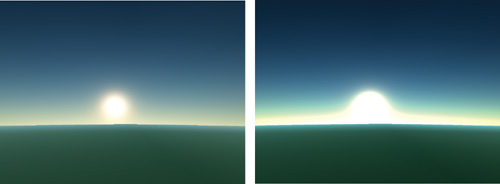
Figure 16-4 The Importance of High Dynamic Range
The exposure equation used in this demo is very simple: 1.0 – exp(-fExposure x color). The exposure constant works like the aperture of a camera or the pupils of your eyes. When there is too much light, the exposure constant is reduced to let in less light. When there is not enough light, the exposure constant is increased to let in more light. Without reasonable limits set on the exposure constant, daylight can look like moonlight and vice versa. Regardless, the relative brightness of each color is always preserved.
The HDR rendering implemented in this demo is also very simple. An OpenGL pbuffer is created with a floating-point pixel format and render-to-texture enabled. The same rendering code as before is used, but everything is rendered to the pbuffer's rendering context. Afterward, the main rendering context is selected and a single quad is rendered to fill the screen. The floating-point buffer is selected as a texture, and a simple exponential scaling shader is used to scale the colors to the normal 0–255 range. The exposure constant is set manually and can be changed at runtime in the demo, along with several of the scattering constants used.
Fortunately, modern GPUs support floating-point render targets. Some critical features such as alpha blending aren't available until you move up to GeForce 6 Series GPUs, so blending the sky dome with objects rendered in space won't work for older GPUs.
16.7 Conclusion
Although it took a fair number of simplifications to be able to interactively render scenes with the model described, the demo looks pretty sharp, especially with HDR rendering. Tweaking the parameters to the system can be a source of much entertainment; I had never imagined that the sky at the horizon would be orange at high noon if our atmosphere were a little thicker, or that sunsets would look that much more incredible. Red and orange skies produce sunsets of different shades of blue, and purple skies produce green sunsets. Once I even managed to find settings that produced a rainbow sunset.
In any case, the work is not done here. There are a number of improvements that could be made to this algorithm:
- Create an atmospheric-density scale function that is not hard-coded to a specific scale height and the ratio between the atmosphere thickness and the planetary radius.
- Split up the Rayleigh and Mie scattering so that they can have different scale depths.
- Provide a better way to simulate multiple scattering and start using the Rayleigh phase function again.
- Allow light from other sources, such as the moon, to be scattered, as well as sunlight. This would be necessary to create a moonlight effect with a halo surrounding the moon.
- Atmospheric scattering also makes distant objects look larger and blurrier than they are. The moon would look much smaller to us if it were not viewed through an atmosphere. It may be possible to achieve this in the HDR pass with some sort of blurring filter that is based on optical depth.
- Change the sample points taken along the ray from linear to exponential based on altitude. Nishita et al. 1993 explains why this is beneficial.
- Add other atmospheric effects, such as clouds, precipitation, lightning, and rainbows. See Harris 2001, Brewer 2004, and Dobashi et al. 2001.
16.8 References
Brewer, Clint. 2004. "Rainbows and Fogbows: Adding Natural Phenomena." NVIDIA Corporation. SDK white paper. http://download.nvidia.com/developer/SDK/Individual_Samples/DEMOS/Direct3D9/src/HLSL_RainbowFogbow/docs/RainbowFogbow.pdf
Dobashi, Y., T. Yamamoto, and T. Nishita. 2001. "Efficient Rendering of Lightning Taking into Account Scattering Effects due to Clouds and Atmospheric Particles." http://nis-lab.is.s.u-tokyo.ac.jp/~nis/cdrom/pg/pg01_lightning.pdf
Harris, Mark J., and Anselmo Lastra. 2001. "Real-Time Cloud Rendering." Eurographics 2001 20(3), pp. 76–84. http://www.markmark.net/PDFs/RTClouds_HarrisEG2001.pdf
Hoffman, N., and A. J. Preetham. 2002. "Rendering Outdoor Scattering in Real Time." ATI Corporation. http://www.ati.com/developer/dx9/ATI-LightScattering.pdf
Nishita, T., T. Sirai, K. Tadamura, and E. Nakamae. 1993. "Display of the Earth Taking into Account Atmospheric Scattering." In Proceedings of SIGGRAPH 93, pp. 175–182. http://nis-lab.is.s.u-tokyo.ac.jp/~nis/cdrom/sig93_nis.pdf
O'Neil, Sean. 2004. "Real-Time Atmospheric Scattering." GameDev.net. http://www.gamedev.net/columns/hardcore/atmscattering/
Copyright
Many of the designations used by manufacturers and sellers to distinguish their products are claimed as trademarks. Where those designations appear in this book, and Addison-Wesley was aware of a trademark claim, the designations have been printed with initial capital letters or in all capitals.
The authors and publisher have taken care in the preparation of this book, but make no expressed or implied warranty of any kind and assume no responsibility for errors or omissions. No liability is assumed for incidental or consequential damages in connection with or arising out of the use of the information or programs contained herein.
NVIDIA makes no warranty or representation that the techniques described herein are free from any Intellectual Property claims. The reader assumes all risk of any such claims based on his or her use of these techniques.
The publisher offers excellent discounts on this book when ordered in quantity for bulk purchases or special sales, which may include electronic versions and/or custom covers and content particular to your business, training goals, marketing focus, and branding interests. For more information, please contact:
U.S. Corporate and Government Sales
(800) 382-3419
corpsales@pearsontechgroup.com
For sales outside of the U.S., please contact:
International Sales
international@pearsoned.com
Visit Addison-Wesley on the Web: www.awprofessional.com
Library of Congress Cataloging-in-Publication Data
GPU gems 2 : programming techniques for high-performance graphics and general-purpose
computation / edited by Matt Pharr ; Randima Fernando, series editor.
p. cm.
Includes bibliographical references and index.
ISBN 0-321-33559-7 (hardcover : alk. paper)
1. Computer graphics. 2. Real-time programming. I. Pharr, Matt. II. Fernando, Randima.
T385.G688 2005
006.66—dc22
2004030181
GeForce™ and NVIDIA Quadro® are trademarks or registered trademarks of NVIDIA Corporation.
Nalu, Timbury, and Clear Sailing images © 2004 NVIDIA Corporation.
mental images and mental ray are trademarks or registered trademarks of mental images, GmbH.
Copyright © 2005 by NVIDIA Corporation.
All rights reserved. No part of this publication may be reproduced, stored in a retrieval system, or transmitted, in any form, or by any means, electronic, mechanical, photocopying, recording, or otherwise, without the prior consent of the publisher. Printed in the United States of America. Published simultaneously in Canada.
For information on obtaining permission for use of material from this work, please submit a written request to:
Pearson Education, Inc.
Rights and Contracts Department
One Lake Street
Upper Saddle River, NJ 07458
Text printed in the United States on recycled paper at Quebecor World Taunton in Taunton, Massachusetts.
Second printing, April 2005
Dedication
To everyone striving to make today's best computer graphics look primitive tomorrow
- Copyright
- Inside Back Cover
- Inside Front Cover
- Part I: Geometric Complexity
-
- Chapter 1. Toward Photorealism in Virtual Botany
- Chapter 2. Terrain Rendering Using GPU-Based Geometry Clipmaps
- Chapter 3. Inside Geometry Instancing
- Chapter 4. Segment Buffering
- Chapter 5. Optimizing Resource Management with Multistreaming
- Chapter 6. Hardware Occlusion Queries Made Useful
- Chapter 7. Adaptive Tessellation of Subdivision Surfaces with Displacement Mapping
- Chapter 8. Per-Pixel Displacement Mapping with Distance Functions
- Part II: Shading, Lighting, and Shadows
-
- Chapter 9. Deferred Shading in S.T.A.L.K.E.R.
- Chapter 10. Real-Time Computation of Dynamic Irradiance Environment Maps
- Chapter 11. Approximate Bidirectional Texture Functions
- Chapter 12. Tile-Based Texture Mapping
- Chapter 13. Implementing the mental images Phenomena Renderer on the GPU
- Chapter 14. Dynamic Ambient Occlusion and Indirect Lighting
- Chapter 15. Blueprint Rendering and "Sketchy Drawings"
- Chapter 16. Accurate Atmospheric Scattering
- Chapter 17. Efficient Soft-Edged Shadows Using Pixel Shader Branching
- Chapter 18. Using Vertex Texture Displacement for Realistic Water Rendering
- Chapter 19. Generic Refraction Simulation
- Part III: High-Quality Rendering
-
- Chapter 20. Fast Third-Order Texture Filtering
- Chapter 21. High-Quality Antialiased Rasterization
- Chapter 22. Fast Prefiltered Lines
- Chapter 23. Hair Animation and Rendering in the Nalu Demo
- Chapter 24. Using Lookup Tables to Accelerate Color Transformations
- Chapter 25. GPU Image Processing in Apple's Motion
- Chapter 26. Implementing Improved Perlin Noise
- Chapter 27. Advanced High-Quality Filtering
- Chapter 28. Mipmap-Level Measurement
- Part IV: General-Purpose Computation on GPUS: A Primer
-
- Chapter 29. Streaming Architectures and Technology Trends
- Chapter 30. The GeForce 6 Series GPU Architecture
- Chapter 31. Mapping Computational Concepts to GPUs
- Chapter 32. Taking the Plunge into GPU Computing
- Chapter 33. Implementing Efficient Parallel Data Structures on GPUs
- Chapter 34. GPU Flow-Control Idioms
- Chapter 35. GPU Program Optimization
- Chapter 36. Stream Reduction Operations for GPGPU Applications
- Part V: Image-Oriented Computing
-
- Chapter 37. Octree Textures on the GPU
- Chapter 38. High-Quality Global Illumination Rendering Using Rasterization
- Chapter 39. Global Illumination Using Progressive Refinement Radiosity
- Chapter 40. Computer Vision on the GPU
- Chapter 41. Deferred Filtering: Rendering from Difficult Data Formats
- Chapter 42. Conservative Rasterization
- Part VI: Simulation and Numerical Algorithms
-
- Chapter 43. GPU Computing for Protein Structure Prediction
- Chapter 44. A GPU Framework for Solving Systems of Linear Equations
- Chapter 45. Options Pricing on the GPU
- Chapter 46. Improved GPU Sorting
- Chapter 47. Flow Simulation with Complex Boundaries
- Chapter 48. Medical Image Reconstruction with the FFT