
GPU Gems 2
GPU Gems 2 is now available, right here, online. You can purchase a beautifully printed version of this book, and others in the series, at a 30% discount courtesy of InformIT and Addison-Wesley.
The CD content, including demos and content, is available on the web and for download.
Chapter 42. Conservative Rasterization
Jon Hasselgren
Lund University
Tomas Akenine-Möller
Lund University
Lennart Ohlsson
Lund University
Over the past few years, general-purpose computation using GPUs has received much attention in the research community. The stream-based rasterization architecture provides for much faster performance growth than that of CPUs, and therein lies the attraction in implementing an algorithm on the GPU: if not now, then at some point in time, your algorithm is likely to run faster on the GPU than on a CPU.
However, some algorithms that discretize their continuous problem domain do not return exact results when the GPU's standard rasterization is used. Examples include algorithms for collision detection (Myzskowski et al. 1995, Govindaraju et al. 2003), occlusion culling (Koltun et al. 2001), and visibility testing for shadow acceleration (Lloyd et al. 2004). The accuracy of these algorithms can be improved by increasing rendering resolution. However, one can never guarantee a fully correct result. This is similar to the antialiasing problem: you can never avoid sampling artifacts by just increasing the number of samples; you can only reduce the problems at the cost of performance.
A simple example of when standard rasterization does not compute the desired result is shown in Figure 42-1a, where one green and one blue triangle have been rasterized. These triangles overlap geometrically, but the standard rasterization process does not detect this fact. With conservative rasterization, the overlap is always properly detected, no matter what resolution is used. This property can enable load balancing between the CPU and the GPU. For example, for collision detection, a lower resolution would result in less work for the GPU and more work for the CPU, which performs exact intersection tests. See Figure 42-1b for the results of using conservative rasterization.
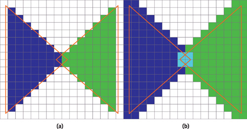
Figure 42-1 Comparing Standard and Conservative Rasterization
There already exists a simple algorithm for conservative rasterization (Akenine-Möller and Aila, forthcoming). However, that algorithm is designed for hardware implementation. In this chapter we present an alternative that is adapted for implementation using vertex and fragment programs on the GPU.
42.1 Problem Definition
In this section, we define what we mean by conservative rasterization of a polygon. First, we define a pixel cell as the rectangular region around a pixel in a pixel grid. There are two variants of conservative rasterization, namely, overestimated and underestimated (Akenine-Möller and Aila, forthcoming):
- An overestimated conservative rasterization of a polygon includes all pixels for which the intersection between the pixel cell and the polygon is nonempty.
- An underestimated conservative rasterization of a polygon includes only the pixels whose pixel cell lies completely inside the polygon.
Here, we are mainly concerned with the overestimated variant, because that one is usually the most useful. If not specified further, we mean the overestimated variant when writing "conservative rasterization."
As can be seen, the definitions are based only on the pixel cell and are therefore independent of the number of sample points for a pixel. To that end, we choose not to consider render targets that use multisampling, because this would be just a waste of resources. It would also further complicate our implementation.
The solution to both of these problems can be seen as a modification of the polygon before the rasterization process. Overestimated conservative rasterization can be seen as the image-processing operation dilation of the polygon by the pixel cell. Similarly, underestimated conservative rasterization is the erosion of the polygon by the pixel cell. Therefore, we transform the rectangle-polygon overlap test of conservative rasterization into a point-in-region test.
The dilation is obtained by locking the center of a pixel-cell-size rectangle to the polygon edges and sweeping it along them while adding all the pixel cells it touches to the dilated triangle. Alternatively, for a convex polygon, the dilation can be computed as the convex hull of a set of pixel cells positioned at each of the vertices of the polygon. This is the equivalent of moving the vertices of the polygon in each of the four possible directions from the center of a pixel cell to its corners and then computing the convex hull. Because the four vectors from the center of a pixel cell to each corner are important in any algorithm for conservative rasterization, we call them the semidiagonals. This type of vertex movement is shown by the green lines in Figure 42-2a, which also shows the bounding polygon for a triangle.
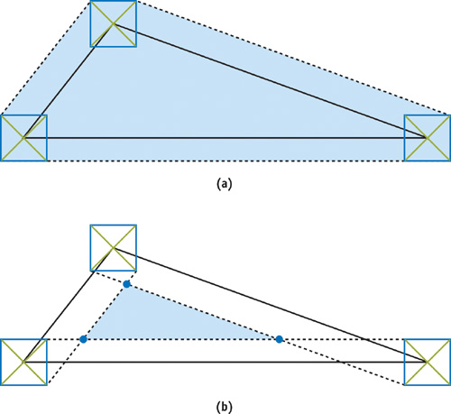
Figure 42-2 Overestimated and Underestimated Rasterization
The erosion is obtained by sweeping the pixel-cell-size rectangle in the same manner as for dilation, but instead we erase all the pixel cells it touches. We note that for a general convex polygon, the number of vertices may be decreased due to this operation. In the case of a triangle, the result will always be a smaller triangle or an "empty" polygon. The erosion of a triangle is illustrated in Figure 42-2b.
42.2 Two Conservative Algorithms
We present two algorithms for conservative rasterization that have different performance characteristics. The first algorithm computes the optimal bounding polygon in a vertex program. It is therefore optimal in terms of fill rate, but it is also costly in terms of geometry processing and data setup, because every vertex must be replicated. The second algorithm computes a bounding triangle—a bounding polygon explicitly limited to only three vertices—in a vertex program and then trims it in a fragment program. This makes it less expensive in terms of geometry processing, because constructing the bounding triangle can be seen as repositioning each of the vertices of the input triangle. However, the bounding triangle is a poor fit for triangles with acute angles; therefore, the algorithm is more costly in terms of fill rate.
To simplify the implementation of both algorithms, we assume that no edges resulting from clipping by the near or far clip planes lie inside the view frustum. Edges resulting from such clipping operations are troublesome to detect, and they are very rarely used for any important purpose in this context.
42.2.1 Clip Space
We describe both algorithms in window space, for clarity, but in practice it is impossible to work in window space, because the vertex program is executed before the clipping and perspective projection. Fortunately, our reasoning maps very simply to clip space. For the moment, let us ignore the z component of the vertices (which is used only to interpolate a depth-buffer value). Doing so allows us to describe a line through each edge of the input triangle as a plane in homogeneous (x c , y c , w c )-space. The plane is defined by the two vertices on the edge of the input triangle, as well as the position of the viewer, which is the origin, (0, 0, 0). Because all of the planes pass through the origin, we get plane equations of the form
|
ax c + by c + cw c
= 0
|
 a(xw c ) + b (yw c ) +
cw c ) + cw c = 0
a(xw c ) + b (yw c ) +
cw c ) + cw c = 0
 ax + by + c = 0
The planes are equivalent to lines in two dimensions. In many of our computations, we use the normal of an edge, which is defined by (a, b) from the plane equation.
42.2.2 The First Algorithm
In this algorithm we compute the optimal bounding polygon for conservative rasterization, shown in Figure 42-2a. Computing the convex hull, from the problem definition section, sounds like a complex task to perform in a vertex program. However, it comes down to three simple cases, as illustrated in Figure 42-3. Given two edges e 1 and e 2 connected in a vertex v, the three cases are the following:
- If the normals of e 1 and e 2 lie in the same quadrant, the convex hull is defined by the point found by moving the vertex v by the semidiagonal in that quadrant (Figure 42-3a).
- If the normals of e 1 and e 2 lie in neighboring quadrants, the convex hull is defined by two points. The points are found by moving v by the semidiagonals in those quadrants (Figure 42-3b).
- If the normals of e 1 and e 2 lie in opposite quadrants, the convex hull is defined by three points. Two points are found as in the previous case, and the last point is found by moving v by the semidiagonal of the quadrant between the opposite quadrants (in the winding order) (Figure 42-3c).
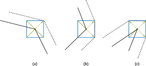
Figure 42-3 Computing an Optimal Bounding Polygon
Implementation
We implement the algorithm as a vertex program that creates output vertices according to the three cases. Because we cannot create vertices in the vertex program, we must assume the worst-case scenario from Figure 42-3c. To create a polygon from a triangle, we must send three instances of each vertex of the input triangle to the hardware and then draw the bounding polygon as a triangle fan with a total of nine vertices. The simpler cases from Figure 42-3, resulting in only one or two vertices, are handled by collapsing two or three instances of a vertex to the same position and thereby generating degenerate triangles. For each instance of every vertex, we must also send the positions of the previous and next vertices in the input triangle, as well as a local index in the range [0,2]. The positions and indices are needed to compute which case and which semidiagonal to use when computing the new vertex position.
The core of the vertex program consists of code that selects one of the three cases and creates an appropriate output vertex, as shown in Listing 42-1.
Example 42-1. Vertex Program Implementing the First Algorithm
// semiDiagonal[0,1] = Normalized semidiagonals in the same
// quadrants as the edge's normals.
// vtxPos = The position of the current vertex.
// hPixel = dimensions of half a pixel cell
float dp = dot(semiDiagonal[0], semiDiagonal[1]);
float2 diag;
if (dp > 0)
{
  // The normals are in the same quadrant->One vertex
  diag = semiDiagonal[0];
}
else if (dp < 0)
{
  // The normals are in neighboring quadrants->Two vertices
  diag = (In.index == 0 ? semiDiagonal[0] : semiDiagonal[1]);
}
else
{
  // The normals are in opposite quadrants->Three vertices
  if (In.index == 1)
  {
    // Special "quadrant between two quadrants case"
    diag = float2(semiDiagonal[0].x * semiDiagonal[0].y * semiDiagonal[1].x,
                  semiDiagonal[0].y * semiDiagonal[1].x * semiDiagonal[1].y);
  }
  else
    diag = (In.index == 0 ? semiDiagonal[0] : semiDiagonal[1]);
}
vtxPos.xy += hPixel.xy * diag * vtxPos.w;
In cases with input triangles that have vertices behind the eye, we can get projection problems that force tessellation edges out of the bounding polygon in its visible regions. To solve this problem, we perform basic near-plane clipping of the current edge. If orthographic projection is used, or if no polygon will intersect the near clip plane, we skip this operation.
42.2.3 The Second Algorithm
The weakness of the first algorithm is that it requires multiple output vertices for each input vertex. An approach that avoids this problem is to compute a bounding triangle for every input triangle, instead of computing the optimal bounding polygon, which may have as many as nine vertices. However, the bounding triangle is a bad approximation for triangles with acute angles. As a result, we get an overly conservative rasterization, as shown in Figure 42-4. The poor fit makes the bounding triangles practically useless. To work around this problem, we use an alternative interpretation of a simple test for conservative rasterization (Akenine-Möller and Aila, forthcoming). The bounding polygon (as used in Section 42.2.2) can be computed as the intersection of the bounding triangle and the axis-aligned bounding box (AABB) of itself. The AABB of the bounding polygon can easily be computed from the input triangle. Figure 42-5 illustrates this process.
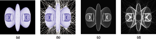
Figure 42-4 Objects Rasterized in Different Ways
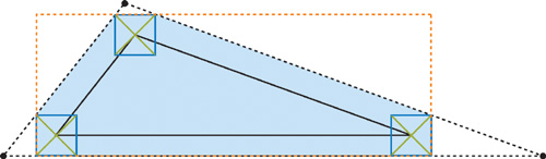
Figure 42-5 An Input Triangle and Its Optimal Bounding Polygon
In our second algorithm, we compute the bounding triangle in a vertex program and then use a fragment program to discard all fragments that do not overlap the AABB.
We can find the three edges of the bounding triangle by computing the normal of the line through each edge of the input triangle and then moving that line by the worst-case semidiagonal. The worst-case semidiagonal is always the one found in the same quadrant as the line normal.
After computing the translated lines, we compute the intersection points of adjacent edges to get the vertices of the bounding triangle. At this point, we can make good use of the clip-space representation. Because each line is represented as a plane through the origin, we can compute the intersection of two planes with normals n 1= (x 1, y 1, w 1) and n 2= (x 2, y 2, w 2) as the cross product n 1 x n 2.
Note that the result is a direction rather than a point, but all points in the given direction will project to the same point in window space. This also ensures that the w component of the computed vertex receives the correct sign.
Implementation
Because the bounding triangle moves every vertex of the input triangle to a new position, we need to send only three vertices for every input triangle. However, along with each vertex, we also send the positions of the previous and next vertices, as texture coordinates, so we can compute the edges. For the edges, we use planes rather than lines. A parametric representation of the lines, in the form of a point and a direction, would simplify the operation of moving the line at the cost of more problems when computing intersection. Because we represent our lines as equations of the form:
|
(a, b) · x + c = 0, |
we must derive how to modify the line equation to represent a movement by a vector v. It can be done by modifying the c component of the line equation as:
|
c moved = c – v · (a, b ). |
If we further note that the problem of finding a semidiagonal is symmetric with respect to 90-degree rotations, we can use a fixed semidiagonal in the first quadrant along with the component-wise absolute values of the line normal to move the line. The code in Listing 42-2 shows the core of the bounding triangle computation.
Example 42-2. Cg Code for Computing the Bounding Triangle
// hPixel = dimensions of half a pixel cell
// Compute equations of the planes through the two edges
float3 plane[2];
plane[0] = cross(currentPos.xyw - prevPos.xyw, prevPos.xyw);
plane[1] = cross(nextPos.xyw - currentPos.xyw, currentPos.xyw);
// Move the planes by the appropriate semidiagonal
plane[0].z -= dot(hPixel.xy, abs(plane[0].xy));
plane[1].z -= dot(hPixel.xy, abs(plane[1].xy));
// Compute the intersection point of the planes.
float4 finalPos;
finalPos.xyw = cross(plane[0], plane[1]);
We compute the screen-space AABB for the optimal bounding polygon in our vertex program. We iterate over the edges of the input triangle and modify the current AABB candidate to include that edge. The result is an AABB for the input triangle. Extending its size by a pixel cell gives us the AABB for the optimal bounding polygon. To guarantee the correct result, we must clip the input triangle by the near clip plane to avoid back projection. The clipping can be removed under the same circumstances as for the previous algorithm.
We send the AABB of the bounding polygon and the clip-space position to a fragment program, where we perform perspective division on the clip-space position and discard the fragment if it lies outside the AABB. The fragment program is implemented by the following code snippet:
// Compute the device coordinates of the current pixel
float2 pos = In.clipSpace.xy / In.clipSpace.w;
// Discard fragment if outside the AABB. In.AABB contains min values
// in the xy components and max values in the zw components
discard(pos.xy<In.AABB.xy || pos.xy> In.AABB.zw);
Underestimated Conservative Rasterization
So far, we have covered algorithms only for overestimated conservative rasterization. However, we have briefly implied that the optimal bounding polygon for underestimated rasterization is a triangle or an "empty" polygon. The bounding triangle for underestimated rasterization can be computed just like the bounding triangle for overestimated rasterization: simply swap the minus for a plus when computing a new c component for the lines. The case of the empty polygon is automatically addressed because the bounding triangle will change winding order and be culled by the graphics hardware.
42.3 Robustness Issues
Both our algorithms have issues that, although not equivalent, suggest the same type of solution. The first algorithm is robust in terms of floating-point errors but may generate front-facing triangles when the bounding polygon is tessellated, even though the input primitive was back-facing. The second algorithm generates bounding triangles with the correct orientation, but it suffers from precision issues in the intersection computations when near-degenerate input triangles are used. Note that degenerate triangles may be the result of projection (with a very large angle between view direction and polygon), rather than a bad input.
To solve these problems, we first assume that the input data contains no degenerate triangles. We introduce a value, e, small enough that we consider all errors caused by e to fall in the same category as other floating-point precision errors. If the signed distance from the plane of the triangle to the viewpoint is less than e, we consider the input triangle to be back-facing and output the vertices expected for standard rasterization. This hides the problems because it allows the GPU's culling unit to remove the back-facing polygons.
42.4 Conservative Depth
When performing conservative rasterization, you often want to compute conservative depth values as well. By conservative depth, we mean either the maximum or the minimum depth values, z max and z min, in each pixel cell. For example, consider a simple collision-detection scenario (Govindaraju et al. 2003) with two objects A and B. If any part of object A is occluded by object B and any part of object B is occluded by object A, we say that the objects potentially collide. To perform the first half of this test using our overestimating conservative rasterizer, we would first render object B to the depth buffer using a computed z min as the depth. We would then render object A with depth writes disabled and occlusion queries enabled, and using a computed z max as depth. If any fragments of object A were discarded during rasterization, the objects potentially collide. This result could be used to initiate an exact intersection point computation on the CPU.
When an attribute is interpolated over a plane covering an entire pixel cell, the extreme values will always be in one of the corners of the cell. We therefore compute z max and z min based on the plane of the triangle, rather than the exact triangle representation. Although this is just an approximation, it is conservatively correct. It will always compute a z max greater than or equal to the exact solution and a z min less than or equal to it. This is illustrated in Figure 42-6.
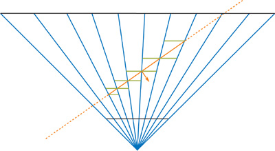
Figure 42-6 Finding the Farthest Depth Value
The depth computation is implemented in our fragment program. A ray is sent from the eye through one of the corners of the current pixel cell. If z max is desired, we send the ray through the corner found in the direction of the triangle normal; the z min depth value can be found in the opposite corner. We compute the intersection point between the ray and the plane of the triangle and use its coordinates to get the depth value. In some cases, the ray may not intersect the plane (or have an intersection point behind the viewer). When this happens, we simply return the maximum depth value.
We can compute the depth value from an intersection point in two ways. We can compute interpolation parameters for the input triangle in the vertex program and then use the intersection point coordinates to interpolate the z (depth) component. This works, but it is computationally expensive and requires many interpolation attributes to transfer the (constant) interpolation base from the vertex program to the fragment program. If the projection matrix is simple, as produced by glFrustum, for instance, it will be of the form:
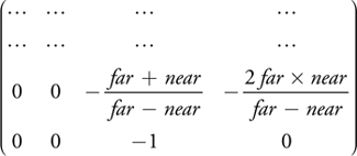
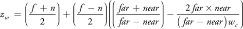
In this case we can use a second, simpler way of computing the depth value. Under the assumption that the input is a normal point with w e = 1 (the eye-space w component), we can compute the z w (window-depth) component of an intersection point from the wc (clip-space w) component. For a depth range [n, f], we compute zw as:
42.5 Results and Conclusions
We have implemented two GPU-accelerated algorithms for conservative rasterization. Both algorithms have strong and weak points, and it is therefore hard to pick a clear winner. As previously stated, the first algorithm is costly in terms of geometry processing, while the second algorithm requires more fill rate. However, the distinction is not that simple. The overdraw complexity of the second algorithm depends both on the acuity of the triangles in a mesh and on the rendering resolution, which controls how far an edge is moved. The extra overdraw caused by the second algorithm therefore depends on the mesh tessellation in proportion to the rendering resolution. Our initial benchmarks in Figure 42-7 show that the first algorithm seems to be more efficient on high-end hardware (such as GeForce 6800 Series GPUs). Older GPUs (such as the GeForce FX 5600) quickly become vertex limited; therefore, the second algorithm may be more suitable in such cases.
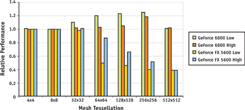
Figure 42-7 Relative Performance of the Two Algorithms
It is likely that the first algorithm will be the better choice in the future. The vertex-processing power of graphics hardware is currently growing faster than the fragment processing power. And with potential future features such as "geometry shaders," we could make a better implementation of the first algorithm.
We can probably enhance the performance of both of our algorithms by doing silhouette edge detection on the CPU and computing bounding polygons only for silhouette edges, or for triangles with at least one silhouette edge. This would benefit the GPU load of both of our algorithms, at the expense of more CPU work.
Our algorithms will always come with a performance penalty when compared to standard rasterization. However, because we can always guarantee that the result is conservatively correct, it is possible that the working resolution can be significantly lowered. In contrast, standard rasterization will sometimes generate incorrect results, which for many applications is completely undesirable.
42.6 References
Akenine-Möller, Tomas, and Timo Aila. Forthcoming. "Conservative and Tiled Rasterization Using a Modified Triangle Setup." Journal of Graphics Tools.
Govindaraju, Naga K., Stephane Redon, Ming C. Lin, and Dinesh Manocha. 2003. "CULLIDE: Interactive Collision Detection Between Complex Models in Large Environments Using Graphics Hardware." In Proceedings of the SIGGRAPH/Eurographics Workshop on Graphics Hardware 2003, pp. 25–32.
Koltun, Vladlen, Daniel Cohen-Or, and Yiorgos Chrysanthou. 2001. "Hardware-Accelerated From-Region Visibility Using a Dual Ray Space." In 12th Eurographics Workshop on Rendering, pp. 204–214.
Lloyd, Brandon, Jeremy Wendt, Naga Govindaraju, and Dinesh Manocha. 2004. "CC Shadow Volumes." In Eurographics Symposium on Rendering 2004, pp. 197–205.
McCormack, Joel, and Robert McNamara. 2000. "Tiled Polygon Traversal Using Half-Plane Edge Functions." In Proceedings of the SIGGRAPH/Eurographics Workshop on Graphics Hardware 2000, pp. 15–21.
Myzskowski, Karol, Oleg G. Okunev, and Tosiyasu L. Kunii. 1995. "Fast Collision Detection Between Complex Solids Using Rasterizing Graphics Hardware." The Visual Computer 11(9), pp. 497–512.
Seitz, Chris. 2004. "Evolution of NV40." Presentation at NVIDIA GPU BBQ 2004. Available online at http://developer.nvidia.com/object/gpu_bbq_2004_presentations.html
Copyright
Many of the designations used by manufacturers and sellers to distinguish their products are claimed as trademarks. Where those designations appear in this book, and Addison-Wesley was aware of a trademark claim, the designations have been printed with initial capital letters or in all capitals.
The authors and publisher have taken care in the preparation of this book, but make no expressed or implied warranty of any kind and assume no responsibility for errors or omissions. No liability is assumed for incidental or consequential damages in connection with or arising out of the use of the information or programs contained herein.
NVIDIA makes no warranty or representation that the techniques described herein are free from any Intellectual Property claims. The reader assumes all risk of any such claims based on his or her use of these techniques.
The publisher offers excellent discounts on this book when ordered in quantity for bulk purchases or special sales, which may include electronic versions and/or custom covers and content particular to your business, training goals, marketing focus, and branding interests. For more information, please contact:
U.S. Corporate and Government Sales
(800) 382-3419
corpsales@pearsontechgroup.com
For sales outside of the U.S., please contact:
International Sales
international@pearsoned.com
Visit Addison-Wesley on the Web: www.awprofessional.com
Library of Congress Cataloging-in-Publication Data
GPU gems 2 : programming techniques for high-performance graphics and general-purpose
computation / edited by Matt Pharr ; Randima Fernando, series editor.
p. cm.
Includes bibliographical references and index.
ISBN 0-321-33559-7 (hardcover : alk. paper)
1. Computer graphics. 2. Real-time programming. I. Pharr, Matt. II. Fernando, Randima.
T385.G688 2005
006.66—dc22
2004030181
GeForce™ and NVIDIA Quadro® are trademarks or registered trademarks of NVIDIA Corporation.
Nalu, Timbury, and Clear Sailing images © 2004 NVIDIA Corporation.
mental images and mental ray are trademarks or registered trademarks of mental images, GmbH.
Copyright © 2005 by NVIDIA Corporation.
All rights reserved. No part of this publication may be reproduced, stored in a retrieval system, or transmitted, in any form, or by any means, electronic, mechanical, photocopying, recording, or otherwise, without the prior consent of the publisher. Printed in the United States of America. Published simultaneously in Canada.
For information on obtaining permission for use of material from this work, please submit a written request to:
Pearson Education, Inc.
Rights and Contracts Department
One Lake Street
Upper Saddle River, NJ 07458
Text printed in the United States on recycled paper at Quebecor World Taunton in Taunton, Massachusetts.
Second printing, April 2005
Dedication
To everyone striving to make today's best computer graphics look primitive tomorrow
- Copyright
- Inside Back Cover
- Inside Front Cover
- Part I: Geometric Complexity
-
- Chapter 1. Toward Photorealism in Virtual Botany
- Chapter 2. Terrain Rendering Using GPU-Based Geometry Clipmaps
- Chapter 3. Inside Geometry Instancing
- Chapter 4. Segment Buffering
- Chapter 5. Optimizing Resource Management with Multistreaming
- Chapter 6. Hardware Occlusion Queries Made Useful
- Chapter 7. Adaptive Tessellation of Subdivision Surfaces with Displacement Mapping
- Chapter 8. Per-Pixel Displacement Mapping with Distance Functions
- Part II: Shading, Lighting, and Shadows
-
- Chapter 9. Deferred Shading in S.T.A.L.K.E.R.
- Chapter 10. Real-Time Computation of Dynamic Irradiance Environment Maps
- Chapter 11. Approximate Bidirectional Texture Functions
- Chapter 12. Tile-Based Texture Mapping
- Chapter 13. Implementing the mental images Phenomena Renderer on the GPU
- Chapter 14. Dynamic Ambient Occlusion and Indirect Lighting
- Chapter 15. Blueprint Rendering and "Sketchy Drawings"
- Chapter 16. Accurate Atmospheric Scattering
- Chapter 17. Efficient Soft-Edged Shadows Using Pixel Shader Branching
- Chapter 18. Using Vertex Texture Displacement for Realistic Water Rendering
- Chapter 19. Generic Refraction Simulation
- Part III: High-Quality Rendering
-
- Chapter 20. Fast Third-Order Texture Filtering
- Chapter 21. High-Quality Antialiased Rasterization
- Chapter 22. Fast Prefiltered Lines
- Chapter 23. Hair Animation and Rendering in the Nalu Demo
- Chapter 24. Using Lookup Tables to Accelerate Color Transformations
- Chapter 25. GPU Image Processing in Apple's Motion
- Chapter 26. Implementing Improved Perlin Noise
- Chapter 27. Advanced High-Quality Filtering
- Chapter 28. Mipmap-Level Measurement
- Part IV: General-Purpose Computation on GPUS: A Primer
-
- Chapter 29. Streaming Architectures and Technology Trends
- Chapter 30. The GeForce 6 Series GPU Architecture
- Chapter 31. Mapping Computational Concepts to GPUs
- Chapter 32. Taking the Plunge into GPU Computing
- Chapter 33. Implementing Efficient Parallel Data Structures on GPUs
- Chapter 34. GPU Flow-Control Idioms
- Chapter 35. GPU Program Optimization
- Chapter 36. Stream Reduction Operations for GPGPU Applications
- Part V: Image-Oriented Computing
-
- Chapter 37. Octree Textures on the GPU
- Chapter 38. High-Quality Global Illumination Rendering Using Rasterization
- Chapter 39. Global Illumination Using Progressive Refinement Radiosity
- Chapter 40. Computer Vision on the GPU
- Chapter 41. Deferred Filtering: Rendering from Difficult Data Formats
- Chapter 42. Conservative Rasterization
- Part VI: Simulation and Numerical Algorithms
-
- Chapter 43. GPU Computing for Protein Structure Prediction
- Chapter 44. A GPU Framework for Solving Systems of Linear Equations
- Chapter 45. Options Pricing on the GPU
- Chapter 46. Improved GPU Sorting
- Chapter 47. Flow Simulation with Complex Boundaries
- Chapter 48. Medical Image Reconstruction with the FFT