
GPU Gems 2
GPU Gems 2 is now available, right here, online. You can purchase a beautifully printed version of this book, and others in the series, at a 30% discount courtesy of InformIT and Addison-Wesley.
The CD content, including demos and content, is available on the web and for download.
Chapter 8. Per-Pixel Displacement Mapping with Distance Functions
William Donnelly
University of Waterloo
In this chapter, we present distance mapping, a technique for adding small-scale displacement mapping to objects in a pixel shader. We treat displacement mapping as a ray-tracing problem, beginning with texture coordinates on the base surface and calculating texture coordinates where the viewing ray intersects the displaced surface. For this purpose, we precompute a three-dimensional distance map, which gives a measure of the distance between points in space and the displaced surface. This distance map gives us all the information necessary to quickly intersect a ray with the surface. Our algorithm significantly increases the perceived geometric complexity of a scene while maintaining real-time performance.
8.1 Introduction
Cook (1984) introduced displacement mapping as a method for adding small-scale detail to surfaces. Unlike bump mapping, which affects only the shading of surfaces, displacement mapping adjusts the positions of surface elements. This leads to effects not possible with bump mapping, such as surface features that occlude each other and nonpolygonal silhouettes. Figure 8-1 shows a rendering of a stone surface in which occlusion between features contributes to the illusion of depth.
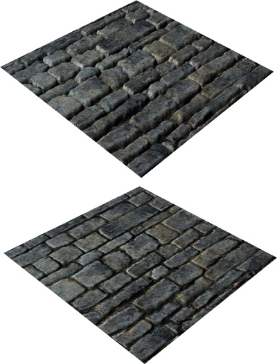
Figure 8-1 A Displaced Stone Surface
The usual implementation of displacement mapping iteratively tessellates a base surface, pushing vertices out along the normal of the base surface, and continuing until the polygons generated are close to the size of a single pixel. Michael Bunnell presents this approach in Chapter 7 of this book, "Adaptive Tessellation of Subdivision Surfaces with Displacement Mapping."
Although it seems most logical to implement displacement mapping in the vertex shading stage of the pipeline, this is not possible because of the vertex shader's inability to generate new vertices. This leads us to consider techniques that rely on the pixel shader. Using a pixel shader is a good idea for several reasons:
- Current GPUs have more pixel-processing power than they have vertex-processing power. For example, the GeForce 6800 Ultra has 16 pixel-shading pipelines to its 6 vertex-shading pipelines. In addition, a single pixel pipeline is often able to perform more operations per clock cycle than a single vertex pipeline.
- Pixel shaders are better equipped to access textures. Many GPUs do not allow texture access within a vertex shader; and for those that do, the access modes are limited, and they come with a performance cost.
- The amount of pixel processing scales with distance. The vertex shader always executes once for each vertex in the model, but the pixel shader executes only once per pixel on the screen. This means work is concentrated on nearby objects, where it is needed most.
A disadvantage of using the pixel shader is that we cannot alter a pixel's screen coordinate within the shader. This means that unlike an approach based on tessellation, an approach that uses the pixel shader cannot be used for arbitrarily large displacements. This is not a severe limitation, however, because displacements are almost always bounded in practice.
8.2 Previous Work
Parallax mapping is a simple way to augment bump mapping to include parallax effects (Kaneko et al. 2001). Parallax mapping uses the information about the height of a surface at a single point to offset the texture coordinates either toward or away from the viewer. Although this is a crude approximation valid only for smoothly varying height fields, it gives surprisingly good results, particularly given that it can be implemented with only three extra shader instructions. Unfortunately, because of the inherent assumptions of the technique, it cannot handle large displacements, high-frequency features, or occlusion between features.
Relief mapping as presented by Policarpo (2004) uses a root-finding approach on a height map. It begins by transforming the viewing ray into texture space. It then performs a linear search to locate an intersection with the surface, followed by a binary search to find a precise intersection point. Unfortunately, linear search requires a fixed step size. This means that in order to resolve small details, it is necessary to increase the number of steps, forcing the user to trade accuracy for performance. Our algorithm does not have this trade-off: it automatically adjusts the step size as necessary to provide fine detail near the surface, while skipping large areas of empty space away from the surface.
View-dependent displacement mapping (Wang et al. 2003) and its extension, generalized displacement mapping (Wang et al. 2004), treat displacement mapping as a ray-tracing problem. They store the result of all possible ray intersection queries within a three-dimensional volume in a five-dimensional map indexed by three position coordinates and two angular coordinates. This map is then compressed by singular value decomposition, and decompressed in a pixel shader at runtime. Because the data is five-dimensional, it requires a significant amount of preprocessing and storage.
The algorithm for displacement rendering we present here is based on sphere tracing (Hart 1996), a technique developed to accelerate ray tracing of implicit surfaces. The concept is the same, but instead of applying the algorithm to ray tracing of implicit surfaces, we apply it to the rendering of displacement maps on the GPU.
8.3 The Distance-Mapping Algorithm
Suppose we want to apply a displacement map to a plane. We can think of the surface as being bounded by an axis-aligned box. The conventional displacement algorithm would render the bottom face of the box and push vertices upward. Our algorithm instead renders the top plane of the box. Then within the shader, we find which point on the displaced surface the viewer would have really seen.
In a sense, we are computing the inverse problem to conventional displacement mapping. Displacement mapping asks, "For this piece of geometry, what pixel in the image does it map to?" Our algorithm asks, "For this pixel in the image, what piece of geometry do we see?" While the first approach is the one used by rasterization algorithms, the second approach is the one used by ray-tracing algorithms. So we approach distance mapping as a ray-tracing problem.
A common ray-tracing approach is to sample the height map at uniformly spaced locations to test whether the viewing ray has intersected the surface. Unfortunately, we encounter the following problem: as long as our samples are spaced farther apart than a single texel, we cannot guarantee that we have not missed an intersection that lies between our samples. This problem is illustrated in Figure 8-2. These "overshoots" can cause gaps in the rendered geometry and can result in severe aliasing. Thus we have two options: either we accept artifacts from undersampling, or we must take a sample for each texel along the viewing ray. Figure 8-3 shows that our algorithm can render objects with fine detail without any aliasing or gaps in geometry.
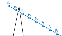
Figure 8-2 A Difficult Case for Displacement Algorithms
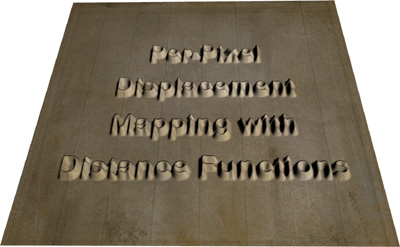
Figure 8-3 Rendering Displaced Text
We can draw two conclusions from the preceding example:
- We cannot simply query the height map at fixed intervals. It either leads to undersampling artifacts or results in an intractable algorithm.
- We need more information at our disposal than just a height field; we need to know how far apart we can take our samples in any given region without overshooting the surface.
To solve these problems, we define the distance map of the surface. For any point p in texture space and a surface S, we define a function dist(p, S) = min{d(p, q) : q in S}. In other words, dist(p, S) is the shortest distance from p to the closest point on the surface S. The distance map for S is then simply a 3D texture that stores, for each point p, the value of dist(p, S). Figure 8-4 shows a sample one-dimensional height map and its corresponding distance map.
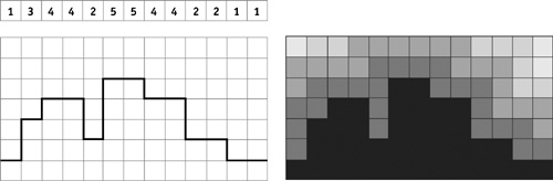
Figure 8-4 A Sample Distance Map in Two Dimensions
This distance map gives us exactly the information we need to choose our sampling positions. Suppose we have a ray with origin p 0 and direction vector d, where d is normalized to unit length. We define a new point p 1= p 0 + dist(p 0, S) x d. This point has the important property that if p 0 is outside the surface, then p 1 is also outside the surface. We then apply the same operation again by defining p 2 = p 1+ dist(p 1, S) xd, and so on. Each consecutive point is a little bit closer to the surface. Thus, if we take enough samples, our points converge toward the closest intersection of the ray with the surface. Figure 8-5 illustrates the effectiveness of this algorithm.
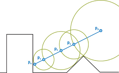
Figure 8-5 Sphere Tracing
It is worth noting that distance functions do not apply only to height fields. In fact, a distance map can represent arbitrary voxelized data. This means that it would be possible to render small-scale detail with complex topology. For example, chain mail could be rendered in this manner.
8.3.1 Arbitrary Meshes
Up to this point, we have discussed applying distance mapping only to planes. We would like to apply distance mapping to general meshes. We do so by assuming the surface is locally planar. Based on this assumption, we can perform the same calculations as in the planar case, using the local tangent frame of the surface. We use the local surface tangents to transform the view vector into tangent space, just as we would transform the light vector for tangent space normal mapping. Once we have transformed the viewing ray into tangent space, the algorithm proceeds exactly as in the planar case.
Now that we know how to use a distance map for ray tracing, we need to know how to efficiently compute a distance map for an arbitrary height field.
8.4 Computing the Distance Map
Computing a distance transform is a well-studied problem. Danielsson (1980) has presented an algorithm that runs in O(n) time, where n is the number of pixels in the map. The idea is to create a 3D map where each pixel stores a 3D displacement vector to the nearest point on the surface. The algorithm then performs a small number of sequential sweeps over the 3D domain, updating each pixel's displacement vector based on neighboring displacement vectors. Once the displacements have been calculated, the distance for each pixel is computed as the magnitude of the displacement. An implementation of this algorithm is on the book's CD.
When the distance transform algorithm is finished, we have computed the distance from each pixel in the distance map to the closest point on the surface, measured in pixels. To make these distances lie in the range [0, 1], we divide each distance by the depth of the 3D texture in pixels.
8.5 The Shaders
8.5.1 The Vertex Shader
The vertex shader for distance mapping, shown in Listing 8-1, is remarkably similar to a vertex shader for tangent-space normal mapping, with two notable differences. The first is that in addition to transforming the light vector into tangent space, we also transform the viewing direction into tangent space. This tangent-space eye vector is used in the vertex shader as the direction of the ray to be traced in texture space. The second difference is that we incorporate an additional factor inversely proportional to the perceived depth. This allows us to adjust the scale of the displacements interactively.
8.5.2 The Fragment Shader
We now have all we need to begin our ray marching: we have a starting point (the base texture coordinate passed down by the vertex shader) and a direction (the tangent-space view vector).
The first thing the fragment shader has to do is to normalize the direction vector. Note that distances stored in the distance map are measured in units proportional to pixels; the direction vector is measured in units of texture coordinates. Generally, the distance map is much higher and wider than it is deep, and so these two measures of distance are quite different. To ensure that our vector is normalized with respect to the measure of distance used by the distance map, we first normalize the direction vector, and then multiply this normalized vector by an extra "normalization factor" of (depth/width, depth/height, 1).
Example 8-1. The Vertex Shader
v2fConnector distanceVertex(a2vConnector a2v, uniform float4x4 modelViewProj,
                            uniform float3 eyeCoord, uniform float3 lightCoord,
                            uniform float invBumpDepth)
{
  v2fConnector v2f;
  // Project position into screen space
  // and pass through texture coordinate
  v2f.projCoord = mul(modelViewProj, float4(a2v.objCoord, 1));
  v2f.texCoord = float3(a2v.texCoord, 1);
  // Transform the eye vector into tangent space.
  // Adjust the slope in tangent space based on bump depth
  float3 eyeVec = eyeCoord - a2v.objCoord;
  float3 tanEyeVec;
  tanEyeVec.x = dot(a2v.objTangent, eyeVec);
  tanEyeVec.y = dot(a2v.objBinormal, eyeVec);
  tanEyeVec.z = -invBumpDepth * dot(a2v.objNormal, eyeVec);
  v2f.tanEyeVec = tanEyeVec;
  // Transform the light vector into tangent space.
  // We will use this later for tangent-space normal mapping
  float3 lightVec = lightCoord - a2v.objCoord;
  float3 tanLightVec;
  tanLightVec.x = dot(a2v.objTangent, lightVec);
  tanLightVec.y = dot(a2v.objBinormal, lightVec);
  tanLightVec.z = dot(a2v.objNormal, lightVec);
  v2f.tanLightVec = tanLightVec;
  return v2f;
}
We can now proceed to march our ray iteratively. We begin by querying the distance map, to obtain a conservative estimate of the distance we can march along the ray without intersecting the surface. We can then step our current position forward by that distance to obtain another point outside the surface. We can proceed in this way to generate a sequence of points that converges toward the displaced surface. Finally, once we have the texture coordinates of the intersection point, we compute normal-mapped lighting in tangent space. Listing 8-2 shows the fragment shader.
8.5.3 A Note on Filtering
When sampling textures, we must be careful about how to specify derivatives for texture lookups. In general, the displaced texture coordinates have discontinuities (for example, due to sections of the texture that are occluded). When mipmapping or anisotropic filtering is enabled, the GPU needs information about the derivatives of the texture coordinates. Because the GPU approximates derivatives with finite differences, these derivatives have incorrect values at discontinuities. This leads to an incorrect choice of mipmap levels, which in turn leads to visible seams around discontinuities.
Instead of using the derivatives of the displaced texture coordinates, we substitute the derivatives of the base texture coordinates. This works because displaced texture coordinates are always continuous, and they vary at approximately the same rate as the base texture coordinates.
Because we do not use the GPU's mechanism for determining mipmap levels, it is possible to have texture aliasing. In practice, this is not a big problem, because the derivatives of the base texture coordinates are a good approximation of the derivatives of the displaced texture coordinates.
Note that the same argument about mipmap levels also applies to lookups into the distance map. Because the texture coordinates can be discontinuous around feature edges, the texture unit will access a mipmap level that is too coarse. This in turn results in incorrect distance values. Our solution is to filter the distance map linearly without any mipmaps. Because the distance map values are never visualized directly, aliasing does not result from the lack of mipmapping here.
8.6 Results
We implemented the distance-mapping algorithm in OpenGL and Cg as well as in Sh (http://www.libsh.org). The images in this chapter were created with the Sh implementation, which is available on the accompanying CD. Because of the large number of dependent texture reads and the use of derivative instructions, the implementation works only on GeForce FX and GeForce 6 Series GPUs.
Example 8-2. The Fragment Shader
f2fConnector distanceFragment(v2fConnector v2f, uniform sampler2D colorTex,
                              uniform sampler2D normalTex,
                              uniform sampler3D distanceTex,
                              uniform float3 normalizationFactor)
{
  f2fConnector f2f;
  // Normalize the offset vector in texture space.
  // The normalization factor ensures we are normalized with respect
  // to a distance which is defined in terms of pixels.
  float3 offset = normalize(v2f.tanEyeVec);
  offset *= normalizationFactor;
  float3 texCoord = v2f.texCoord;
  // March a ray
  for (int i = 0; i < NUM_ITERATIONS; i++)
  {
    float distance = f1tex3D(distanceTex, texCoord);
    texCoord += distance * offset;
  }
  // Compute derivatives of unperturbed texcoords.
  // This is because the offset texcoords will have discontinuities
  // which lead to incorrect filtering.
  float2 dx = ddx(v2f.texCoord.xy);
  float2 dy = ddy(v2f.texCoord.xy);
  // Do bump-mapped lighting in tangent space.
  // 'normalTex' stores tangent-space normals remapped
  // into the range [0, 1].
  float3 tanNormal = 2 * f3tex2D(normalTex, texCoord.xy, dx, dy) - 1;
  float3 tanLightVec = normalize(v2f.tanLightVec);
  float diffuse = dot(tanNormal, tanLightVec);
  // Multiply diffuse lighting by texture color
  f2f.COL.rgb = diffuse * f3tex2D(colorTex, texCoord.xy, dx, dy);
  f2f.COL.a = 1;
  return f2f;
}
In all examples in this chapter, we have used a 3D texture size of 256x256x16, but this choice may be highly data-dependent. We also experimented with maps up to 512x512x32 for complex data sets. We set the value of NUM_ITERATIONS to 16 iterations for our examples. In most cases, this was more than sufficient, with 8 iterations sufficing for smoother data sets.
Our fragment shader, assuming 16 iterations, compiles to 48 instructions for the GeForce FX. Each iteration of the loop takes 2 instructions: a texture lookup followed by a multiply-add. GeForce FX and GeForce 6 Series GPUs can execute this pair of operations in a single clock cycle, meaning that each iteration takes only one clock cycle. It should be noted that each texture lookup depends on the previous one; on GPUs that limit the number of indirect texture operations, this shader needs to be broken up into multiple passes.
We tested our distance-mapping implementation on a GeForce FX 5950 Ultra and on a GeForce 6800 GT with several different data sets. One such data set is pictured in Figure 8-6. On the GeForce FX 5950 Ultra, we can shade every pixel at 1024x768 resolution at approximately 30 frames per second. If we reduce the number of iterations to 8, we obtain approximately 75 frames per second at the same resolution. On the GeForce 6800 GT, we were able to run at a consistent 70 frames per second, even shading every pixel at 1280x1024 resolution with 16 iterations.
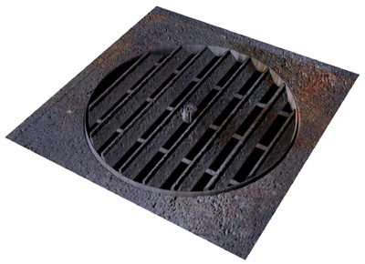
Figure 8-6 A Grating Rendered with Displacement Mapping
8.7 Conclusion
We have presented distance mapping, a fast iterative technique for displacement mapping based on ray tracing of implicit surfaces. We show that the information contained in a distance function allows us to take larger steps when rays are farther from the surface, while ensuring that we never take a step so large that we create gaps in the rendered geometry. The resulting implementation is very efficient; it converges in a few iterations, and each iteration costs only a single cycle on GeForce FX and GeForce 6 Series GPUs.
In the future we would like to use the dynamic branching capabilities of Shader Model 3 GPUs to improve the performance of our technique by taking "early outs" for pixels that converge quickly. This would allow us to increase the quality of the technique by devoting more computing power to pixels that converge more slowly.
We would also like to adapt our technique to curved surfaces. Although our algorithm can be used on any model with appropriate tangents, it results in distortion in regions of high curvature. In particular, generalized displacement mapping (Wang et al. 2004) uses a type of tetrahedral projection to account for curved surfaces, and this method can also be applied to our algorithm. Such a tetrahedral projection can be accomplished in a vertex shader (Wylie et al. 2002).
8.8 References
Cook, Robert L. 1984. "Shade Trees." In Computer Graphics (Proceedings of SIGGRAPH 84) 18(3), pp. 223–231.
Danielsson, Per-Erik. 1980. "Euclidean Distance Mapping." Computer Graphics and Image Processing 14, pp. 227–248.
Hart, John C. 1996. "Sphere Tracing: A Geometric Method for the Antialiased Ray Tracing of Implicit Surfaces." The Visual Computer 12(10), pp. 527–545.
Kaneko, Tomomichi, Toshiyuki Takahei, Masahiko Inami, Naoki Kawakami, Yasuyuki Yanagida, Taro Maeda, and Susumu Tachi. 2001. "Detailed Shape Representation with Parallax Mapping." In Proceedings of the ICAT 2001 (The 11th International Conference on Artificial Reality and Telexistence), Tokyo, December 2001, pp. 205–208.
Policarpo, Fabio. 2004. "Relief Mapping in a Pixel Shader Using Binary Search." http://www.paralelo.com.br/arquivos/ReliefMapping.pdf
Wang, Lifeng, Xi Wang, Xin Tong, Stephen Lin, Shimin Hu, Baining Guo, and Heung-Yeung Shum. 2003. "View-Dependent Displacement Mapping." ACM Transactions on Graphics (Proceedings of SIGGRAPH 2003) 22(3), pp. 334–339.
Wang, Xi, Xin Tong, Stephen Lin, Shimin Hu, Baining Guo, and Heung-Yeung Shum. 2004. "Generalized Displacement Maps." In Eurographics Symposium on Rendering 2004, pp. 227–234.
Wylie, Brian, Kenneth Moreland, Lee Ann Fisk, and Patricia Crossno. 2002. "Tetrahedral Projection Using Vertex Shaders." In Proceedings of IEEE Volume Visualization and Graphics Symposium 2002, October 2002, pp. 7–12.
Special thanks to Stefanus Du Toit for his help implementing the distance transform and writing the Sh implementation.
Copyright
Many of the designations used by manufacturers and sellers to distinguish their products are claimed as trademarks. Where those designations appear in this book, and Addison-Wesley was aware of a trademark claim, the designations have been printed with initial capital letters or in all capitals.
The authors and publisher have taken care in the preparation of this book, but make no expressed or implied warranty of any kind and assume no responsibility for errors or omissions. No liability is assumed for incidental or consequential damages in connection with or arising out of the use of the information or programs contained herein.
NVIDIA makes no warranty or representation that the techniques described herein are free from any Intellectual Property claims. The reader assumes all risk of any such claims based on his or her use of these techniques.
The publisher offers excellent discounts on this book when ordered in quantity for bulk purchases or special sales, which may include electronic versions and/or custom covers and content particular to your business, training goals, marketing focus, and branding interests. For more information, please contact:
U.S. Corporate and Government Sales
(800) 382-3419
corpsales@pearsontechgroup.com
For sales outside of the U.S., please contact:
International Sales
international@pearsoned.com
Visit Addison-Wesley on the Web: www.awprofessional.com
Library of Congress Cataloging-in-Publication Data
GPU gems 2 : programming techniques for high-performance graphics and general-purpose
computation / edited by Matt Pharr ; Randima Fernando, series editor.
p. cm.
Includes bibliographical references and index.
ISBN 0-321-33559-7 (hardcover : alk. paper)
1. Computer graphics. 2. Real-time programming. I. Pharr, Matt. II. Fernando, Randima.
T385.G688 2005
006.66—dc22
2004030181
GeForce™ and NVIDIA Quadro® are trademarks or registered trademarks of NVIDIA Corporation.
Nalu, Timbury, and Clear Sailing images © 2004 NVIDIA Corporation.
mental images and mental ray are trademarks or registered trademarks of mental images, GmbH.
Copyright © 2005 by NVIDIA Corporation.
All rights reserved. No part of this publication may be reproduced, stored in a retrieval system, or transmitted, in any form, or by any means, electronic, mechanical, photocopying, recording, or otherwise, without the prior consent of the publisher. Printed in the United States of America. Published simultaneously in Canada.
For information on obtaining permission for use of material from this work, please submit a written request to:
Pearson Education, Inc.
Rights and Contracts Department
One Lake Street
Upper Saddle River, NJ 07458
Text printed in the United States on recycled paper at Quebecor World Taunton in Taunton, Massachusetts.
Second printing, April 2005
Dedication
To everyone striving to make today's best computer graphics look primitive tomorrow
- Copyright
- Inside Back Cover
- Inside Front Cover
- Part I: Geometric Complexity
-
- Chapter 1. Toward Photorealism in Virtual Botany
- Chapter 2. Terrain Rendering Using GPU-Based Geometry Clipmaps
- Chapter 3. Inside Geometry Instancing
- Chapter 4. Segment Buffering
- Chapter 5. Optimizing Resource Management with Multistreaming
- Chapter 6. Hardware Occlusion Queries Made Useful
- Chapter 7. Adaptive Tessellation of Subdivision Surfaces with Displacement Mapping
- Chapter 8. Per-Pixel Displacement Mapping with Distance Functions
- Part II: Shading, Lighting, and Shadows
-
- Chapter 9. Deferred Shading in S.T.A.L.K.E.R.
- Chapter 10. Real-Time Computation of Dynamic Irradiance Environment Maps
- Chapter 11. Approximate Bidirectional Texture Functions
- Chapter 12. Tile-Based Texture Mapping
- Chapter 13. Implementing the mental images Phenomena Renderer on the GPU
- Chapter 14. Dynamic Ambient Occlusion and Indirect Lighting
- Chapter 15. Blueprint Rendering and "Sketchy Drawings"
- Chapter 16. Accurate Atmospheric Scattering
- Chapter 17. Efficient Soft-Edged Shadows Using Pixel Shader Branching
- Chapter 18. Using Vertex Texture Displacement for Realistic Water Rendering
- Chapter 19. Generic Refraction Simulation
- Part III: High-Quality Rendering
-
- Chapter 20. Fast Third-Order Texture Filtering
- Chapter 21. High-Quality Antialiased Rasterization
- Chapter 22. Fast Prefiltered Lines
- Chapter 23. Hair Animation and Rendering in the Nalu Demo
- Chapter 24. Using Lookup Tables to Accelerate Color Transformations
- Chapter 25. GPU Image Processing in Apple's Motion
- Chapter 26. Implementing Improved Perlin Noise
- Chapter 27. Advanced High-Quality Filtering
- Chapter 28. Mipmap-Level Measurement
- Part IV: General-Purpose Computation on GPUS: A Primer
-
- Chapter 29. Streaming Architectures and Technology Trends
- Chapter 30. The GeForce 6 Series GPU Architecture
- Chapter 31. Mapping Computational Concepts to GPUs
- Chapter 32. Taking the Plunge into GPU Computing
- Chapter 33. Implementing Efficient Parallel Data Structures on GPUs
- Chapter 34. GPU Flow-Control Idioms
- Chapter 35. GPU Program Optimization
- Chapter 36. Stream Reduction Operations for GPGPU Applications
- Part V: Image-Oriented Computing
-
- Chapter 37. Octree Textures on the GPU
- Chapter 38. High-Quality Global Illumination Rendering Using Rasterization
- Chapter 39. Global Illumination Using Progressive Refinement Radiosity
- Chapter 40. Computer Vision on the GPU
- Chapter 41. Deferred Filtering: Rendering from Difficult Data Formats
- Chapter 42. Conservative Rasterization
- Part VI: Simulation and Numerical Algorithms
-
- Chapter 43. GPU Computing for Protein Structure Prediction
- Chapter 44. A GPU Framework for Solving Systems of Linear Equations
- Chapter 45. Options Pricing on the GPU
- Chapter 46. Improved GPU Sorting
- Chapter 47. Flow Simulation with Complex Boundaries
- Chapter 48. Medical Image Reconstruction with the FFT