
GPU Gems 2
GPU Gems 2 is now available, right here, online. You can purchase a beautifully printed version of this book, and others in the series, at a 30% discount courtesy of InformIT and Addison-Wesley.
The CD content, including demos and content, is available on the web and for download.
Chapter 7. Adaptive Tessellation of Subdivision Surfaces with Displacement Mapping
Michael Bunnell
NVIDIA Corporation
In this chapter we describe how to perform view-dependent, adaptive tessellation of Catmull-Clark subdivision surfaces with optional displacement mapping. We use the GPU to do the tessellation calculations, which saves graphics bus bandwidth and is many times faster than using the CPU. The first part of this chapter explains how to tessellate subdivision surfaces to polygons for rendering high-quality curved surfaces without visible polygon artifacts. The second part of this chapter describes how to add displacement-mapping support for rendering highly detailed models that can be animated in real time.
This chapter takes a repeated subdivision approach to tessellation, implemented by rendering into 2D textures. The subdivision, flatness test, and final vertex attribute calculations are done using fragment programs (pixel shaders). This method assumes that the vertex data of the subdivision surface control mesh are stored in a texture map. Intermediate results are also rendered to and read from texture maps, and the final tessellation results (position, normal, and so on) are rendered to a vertex array ready to be used by a render-primitives call such as glDrawElements().
7.1 Subdivision Surfaces
Subdivision surfaces are arguably the most popular curved-surface representation used in computer graphics today. Specifically, Catmull-Clark subdivision surfaces are supported in practically every 3D modeling and animation application. Introduced to the big screen by Pixar with A Bug's Life, they have been used in all of Pixar's movies since, including Finding Nemo and The Incredibles. Subdivision surfaces are often combined with displacement mapping to add extra detail for computer-generated characters in live-action movies. The most striking example of a displacement-mapped subdivision surface model is probably the creature Gollum from the recent Lord of the Rings movies.
Subdivision surfaces are curved surfaces (or higher-order surfaces) described by a simple polygon control mesh and some subdivision rules. The subdivision rules define how to perform one subdivision step on the surface. Each subdivision step creates a new mesh with more geometry and a smoother appearance than the previous mesh. Figure 7-1 illustrates such rules applied to a cube.
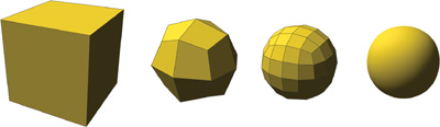
Figure 7-1 Catmull-Clark Subdivision of a Cube
7.1.1 Some Definitions
- Limit surface—the hypothetical surface created after an infinite number of subdivision steps
- Valence (of a vertex)—the number of edges connected to a vertex
- Extraordinary point—a vertex with a valence other than 4 (for a quad-based subdivision scheme, such as Catmull-Clark)
7.1.2 Catmull-Clark Subdivision
We use Catmull-Clark subdivision surfaces in this chapter, and so we use the Catmull-Clark subdivision rules (Catmull and Clark 1978). Catmull-Clark subdivision works on meshes of arbitrary manifold topology. However, it is considered a quad-based subdivision scheme because it works best on four-sided polygons (quads) and because all the polygons in the mesh after the first subdivision step are quads. Our implementation is limited to control meshes consisting only of quads. This implies that the source models have to be created as all-quad models, a task familiar to artists with a NURBS modeling background or experience using Lightwave SubPatches.
The Catmull-Clark rules to subdivide an all-quad mesh are simple. Split each face of the control mesh into four faces by adding a vertex in the middle of the face and a vertex at each edge. The positions of these new vertices and the new positions of the original vertices can be computed from the pre-subdivided mesh vertex positions using the weight masks in Figure 7-2. We show only the weight masks for calculating the new positions of original vertices of valence 3, 4, and 5. The weight masks for higher valences follow the same progression.
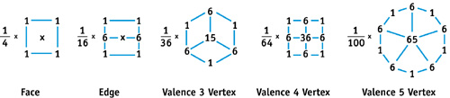
Figure 7-2 Catmull-Clark Subdivision Masks
If we examine a couple of subdivision steps of a single face, we notice that subdivision is very similar to scaling a 2D image. The only differences are the filtering values used and that the vertex position data is generally stored as floating point, while most images are stored as integer or fixed point. Figure 7-3 shows a single face of a mesh being subdivided two times. One thing to note about this figure is that we need a ring of vertices around the faces that are being subdivided to perform the subdivision. Also, the extraordinary point (the vertex of valence 5) at the upper-left corner of the face in the original mesh is present in the subdivided meshes too.
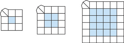
Figure 7-3 Subdividing a Face of a Subdivision Surface
7.1.3 Using Subdivision for Tessellation
One obvious way to tessellate subdivision surfaces is to apply a fixed number of subdivision steps on the original control mesh to create a list of quads to render. In fact, that is how pre-tessellated surfaces are created with most 3D-modeling packages. The disadvantage of this method is that parts of a model are over-tessellated and other parts under-tessellated. Also, it leaves the burden of selecting the number of subdivisions on the application program. Under-tessellation leads to visible polygon artifacts. Over-tessellation creates too many small triangles that can severely affect rendering performance. Too much geometry causes the GPU to become vertex-transform or triangle-setup limited. Worse, having many tiny triangles that are just a few pixels in size can significantly reduce rasterizer efficiency.
Adaptive Subdivision
We use a flatness-test-based adaptive subdivision algorithm to avoid the problems with the fixed subdivision method. Instead of blindly subdividing a fixed number of steps, we test the surface for flatness first. In this way, the subdivision adapts to the surface curvature and the viewpoint. The closer the surface is or the more curved it is, the more it gets subdivided. See Figure 7-4. We measure flatness as the distance from the polygonal mesh to the limit surface measured in screen pixels. For example, a flatness value of 0.5 means the maximum distance from the polygon approximation of the surface to the limit surface is half a pixel.
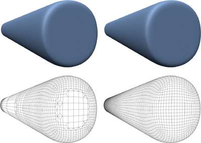
Figure 7-4 Adaptive vs. Uniform Tessellation
7.1.4 Patching the Surface
We need to store the subdivision control mesh vertex data in a format that allows for efficient processing. We do this by breaking up the original control mesh into smaller meshes that can be represented as regular 2D grids and therefore stored in 2D arrays. See Figure 7-5. Now we can infer the mesh connectivity by the location of vertices in the array. Vertices next to each other are assumed to be connected by edges. Control points arranged this way, in a 2D array or matrix, are generally referred to as patches, so that is what we call them. Our patches are different in that we allow extraordinary points at the patches' corners.
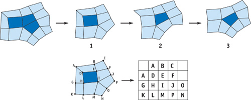
Figure 7-5 Patching a Surface
The obvious way to divide the control mesh into patches is to create a patch for each face of the mesh. This method requires a lot of duplicated vertices because we need to include the vertices from neighboring faces so we can subdivide the patch. We can improve on this situation by creating patches with more faces when possible.
Patching a surface is not a trivial process, but fortunately it can be done in a preprocessing step. Even animated meshes generally do not change topology, so the vertex locations in each patch can be precalculated and stored in a 2D texture. The texture can be passed to the tessellation code along with the list of patch information, which includes the size of the patch and the valences of any extraordinary vertices. The demo program available on the book's Web site shows one possible implementation of patching an arbitrary quad model.
7.1.5 The GPU Tessellation Algorithm
The tessellation algorithm works as follows. First, we copy the vertex data of the control mesh (positions) into the patch buffer texture. The flatness test assumes the vertex coordinates are in eye space. If they are not in eye space, they can be transformed before or during this copy. Next, we check each patch for flatness (see "The Flatness Test," later in this section). Then we compute vertex attribute data, such as positions and normals, for the patches that are flat and write them to the vertex array, writing the index information to a primitive index buffer. Patches that are not flat are subdivided into another patch buffer. Then we swap patch-buffer pointers and go back to the flatness test step. This section describes each step in the tessellation process in more detail.
CPU Processing
We use the CPU to do buffer management and to create the list of vertex indices that form part of the tessellation result. The CPU does not have to touch the vertex data, but it does read the flatness test results (using glReadPixels) and decides which patches need further tessellation. It assigns patch locations in the buffers, and it uses a simple recursive procedure to build the primitive index list based on the edge flatness results computed by the shaders.
Creating the Patches
Patches are created by rendering a quad per patch at the appropriate location in the patch buffer, to copy the control mesh vertex position data from a texture. The program executed at the quad's fragments uses a precomputed texture to index the control mesh vertices discussed in Section 7.1.4. If there are more vertex attributes to subdivide, such as texture coordinates, they are copied into a different location in the patch buffer. Vertex attributes other than position are bilinearly interpolated for performance.
The Flatness Test
The flatness of each edge in the patch is calculated by rendering a quad of appropriate size into the flatness buffer using the FlatTest1.cg or the FlatTest2.cg shaders. (All of the shaders mentioned here can be found with the SubdViewer demo program.) Unlike the other buffers used for tessellation, this buffer is not floating point. It is an 8-bit-per-component buffer.
The two flat-test shaders measure the flatness at each edge of the control mesh. Both shaders treat the four control points along an edge as a b-spline curve and measure the flatness of the curve. One shader is used before the first subdivision step because it can handle s-type curves, which are curves whose first derivatives change sign. The second, faster test is used thereafter, because there are only c-type curves after the first subdivision. (C-type curves have first derivatives that do not change sign and thus are c-shaped.)
As shown in Figure 7-6, the first shader's flatness test calculates the distance from the control point 2 to the midpoint of control points 1 and 3, as well as the distance of control point 3 to the midpoint of control points 2 and 4. The second flatness test calculates the distance from the midpoint of control points 1 and 4 to the midpoint of control points 2 and 3. Both tests compare the calculated distance to the flatness value given in pixels, scaled appropriately. The flatness value is prescaled to account for the distance of the b-spline control points from the limit curve, and it is doubled so the midpoint calculations can be done with only an add. Because the control points are assumed to be in eye space, the flatness distance is scaled by the z value of the midpoint of control points 2 and 3 to handle perspective projection.
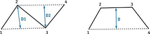
Figure 7-6 Comparing Flatness Tests
The flatness test also needs to handle z-scale values that are less than the near render plane to avoid over-tessellating meshes that cross the near plane. It does so by reflecting z values less than the near plane to the other side of the plane. This technique results in good tessellation for patches that cross the near plane without creating too much geometry that would be clipped later.
Results of the flatness test are copied to host memory, so that the CPU can decide which patches are flat. The results are also saved for each level of subdivision except the last (we know all edges are flat after the last subdivision), so they can be used to build the array of primitive indices. This data is packed to save bandwidth and averages about 200 times fewer bytes of data than the description of the patch itself.
Subdivision
Subdivision is performed by rendering a quad for each patch into the destination patch buffer using the Subdiv.cg shader shown in Listing 7-1. The render works similar to a 2 x scaled image blit, but it uses the weights for Catmull-Clark subdivision, as discussed in Section 7.1.2. The source coordinate for rendering is offset from the patch's origin by (0.75, 0.75), to account for the ring of extra vertices around the faces that are being subdivided and to create a similar ring in the destination. See Figure 7-7. The size of the result patch is twice that of the source patch, minus 3. The Subdiv.cg shader uses the fractional part of the source coordinates to determine which subdivision mask to use: the face mask, the edge mask, or the valence-4 vertex mask. Attributes other than position are interpolated bilinearly in Normal.cg.
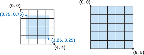
Figure 7-7 Resampling a Patch
Example 7-1. Subdiv.cg—Subdividing a Regular Mesh Using Catmull-Clark Rules
float4 main(float4 srcCoord, uniform samplerRECT srcTexMap : TEXUNIT0) : COLOR
{
  float3 wh, wv;
  // weight values
  float3 s1, s2, s3;
  float2 f;
  // calculate weights based on fractional part of
  // source texture coordinate
  //
  // x == 0.0, y == 0.0 use face weights (1/4, 1/4, 0)
  //
  (1 / 4, 1.4, 0)
      //
      (0, 0, 0)
      // x == 0.5, y == 0.0 use edge weights (horizontal)
      //
      (1 / 16, 6 / 16, 1 / 16)
      //
      (1 / 16, 6 / 16, 1 / 16)
      //
      (0, 0, 0)
      // x == 0.0, y == 0.5 use edge weights (vertical)
      //
      (1 / 16, 1 / 16, 0)
      //
      (6 / 16, 6 / 16, 0)
      //
      (1 / 16, 1 / 16, 0)
      // x == 0.5, y == 0.5 use valence 4 vertex weights
      //
      (1 / 64, 6 / 64, 1 / 64)
      //
      (6 / 64, 36 / 64, 6 / 64)
      //
      (1 / 64, 6 / 64, 1 / 64) wh = float3(1.0 / 8.0, 6.0 / 8.0, 1.0 / 8.0);
  f = frac(srcCoord.xy + 0.001) < 0.25; // account for finite precision
  if (f.x != 0.0)
  {
    wh = float3(0.5, 0.5, 0.0);
    srcCoord.x += 0.5; // fraction was zero -- move to texel center
  }
  wv = float3(1.0 / 8.0, 6.0 / 8.0, 1.0 / 8.0);
  if (f.y != 0)
  {
    wv = float3(0.5, 0.5, 0.0);
    srcCoord.y += 0.5;
    // fraction was zero -- need to move to texel center
  }
  // calculate the destination vertex position by using the weighted
  // sum of the 9 vertex positions centered at srcCoord
  s1 = texRECT(srcTexMap, srcCoord.xy + float2(-1, -1)).xyz * wh.x +
       texRECT(srcTexMap, srcCoord.xy + float2(0, -1)).xyz * wh.y +
       texRECT(srcTexMap, srcCoord.xy + float2(1, -1)).xyz * wh.z;
  s2 = texRECT(srcTexMap, srcCoord.xy + float2(-1, 0)).xyz * wh.x +
       texRECT(srcTexMap, srcCoord.xy + float2(0, 0)).xyz * wh.y +
       texRECT(srcTexMap, srcCoord.xy + float2(1, 0)).xyz * wh.z;
  s3 = texRECT(srcTexMap, srcCoord.xy + float2(-1, 1)).xyz * wh.x +
       texRECT(srcTexMap, srcCoord.xy + float2(0, 1)).xyz * wh.y +
       texRECT(srcTexMap, srcCoord.xy + float2(1, 1)).xyz * wh.z;
  return float4(s1 * wv.x + s2 * wv.y + s3 * wv.z, 0);
}
If there are any extraordinary points at the corners of the patch, they are copied and adjusted using the extraordinary-point subdivision shader, EPSubdiv.cg. This shader does not really subdivide per se, because no more data is created. It only adjusts the positions based on the subdivision rules, using a table lookup to get the appropriate filter weights. It calculates the coordinates of the weights in the lookup table based on the valence of the extraordinary point and the relative position of the control point that it is calculating. This shader is much slower than the regular subdivision shader, but it runs at many fewer pixels. Each corner of the patch (that has an extraordinary point) is handled by rendering a separate, small quad. The extraordinary-point shader is run after the regular subdivision shader and overwrites the control points in the destination that were calculated incorrectly.
Limit Positions and Normals
We use the limit shaders and normal shaders to create the vertex attributes that are written to the vertex array for rendering, including the attributes that are bilinearly interpolated, which are copied in the normal shader. The limit shader calculates the position on the limit surface corresponding to the vertices of the patch. It uses a weighted average of each vertex and its eight neighbors (Halstead et al. 1993). The control points themselves are often not close enough to the limit surface to be substituted for the limit surface points, especially for neighboring patches that are subdivided to different depths. The EPLimit.cg shader is used to calculate the limit position for extraordinary points.
The normal shader calculates two tangents for each control point and then uses their cross product to calculate the surface normal of the limit surface at that point. The EPNormal.cg shader does the same for extraordinary points. Both shaders calculate the tangents using a weighted average of the control vertex's neighbors. Because the normal shaders use the same control points as the limit shaders, it is a good idea to combine them in a single shader and use multiple render targets to write out the position and normal at the same time.
7.1.6 Watertight Tessellation
Watertight tessellation means that there are no gaps between polygons in the tessellation output. Even tiny gaps can lead to missing pixels when rendering the surface. One source of these gaps is the fact that floating-point operations performed in different orders do not always give the exact same result. Ordering shader calculations so that they are identical for neighboring patches costs a lot of performance. Therefore, we do not rely on positions or flatness data at the edge of a patch to match its neighbor's. The index list-building code ensures watertightness by using only one patch's data for shared corners and edges.
Another watertight tessellation problem that must be avoided is T-junctions. T-junctions often crop up with adaptive tessellation schemes. They occur if a patch is split even though one or more of its edges is flat. If the patch sharing the flat edges is not also split, then a T-junction is created. There are different methods for avoiding T-junctions during tessellation, some of which are quite complicated. Our tessellator has the advantage that index values of all the vertices of a patch are known when building the index list. The tessellator simply replaces the index of the vertex at the junction with one that is farther from the edge and fills the gap with a triangle, as illustrated in Figure 7-8. Moving the vertex at the T-junction avoids zero-area triangles, which can cause artifacts when rendering alpha-blended surfaces.
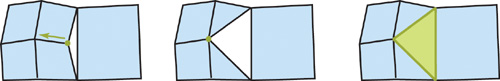
Figure 7-8 Handling T-Junctions
7.2 Displacement Mapping
Displacement mapping is a method for adding geometric complexity to a simple, lightweight model. A displacement map is a texture map containing a scalar value per texel that describes how much the surface to which it is applied should be displaced in the direction of its normal. Unlike bump or normal maps, displacement maps change the actual geometry of the surface, not just the surface normal.
There are several reasons to add displacement mapping to subdivision surfaces. First, subdivision surfaces provide a nice, smooth surface from which to displace, even when animated. Second, they are very compact. The control mesh does not need any normal and tangent data, like polygon models, because they are derived during tessellation. Third, it is easy to modify our subdivision surface shaders to support adaptive displacement mapping.
7.2.1 Changing the Flatness Test
The trick to efficient displacement mapping is adding geometry where it is really needed. We can modify our flatness test so that more geometry is added if the maximum displacement is greater than the flatness threshold. Because the flatness is tested per edge, we create a table using the displacement map containing the maximum displacement on either side of each edge. Figure 7-9 shows a 2D representation of how the maximum distance is calculated for each level of subdivision. Note that all the low-resolution mesh points are located on the displaced surface, because that is where the tessellated vertices are positioned. In the flatness-test shaders, we add the edge's maximum displacement value to the error distance before comparing it to the flatness threshold. All that is left to do geometry-wise is to add the displacement from the displacement map to the vertex position in the limit shaders.
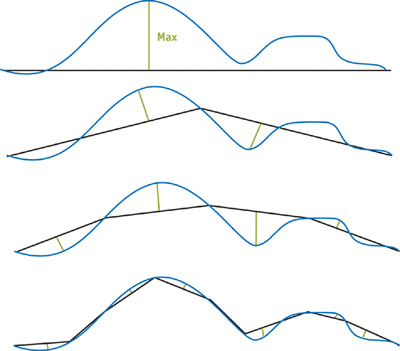
Figure 7-9 Four Steps of the Maximum Displacement Calculation
7.2.2 Shading Using Normal Mapping
We use normal mapping to take the displacement into account when shading the surface, instead of adjusting the vertex normals. See Figure 7-10 for an example. This technique has a couple of advantages. First, normal mapping is done per pixel, so it generally allows more detailed shading than is possible with vertex normals. More important, the surface does not appear to pop when animated, as the amount of geometry changes due to adaptive tessellation. Normal mapping requires some extra attributes from the tessellator: a tangent, and normal map texture coordinates.
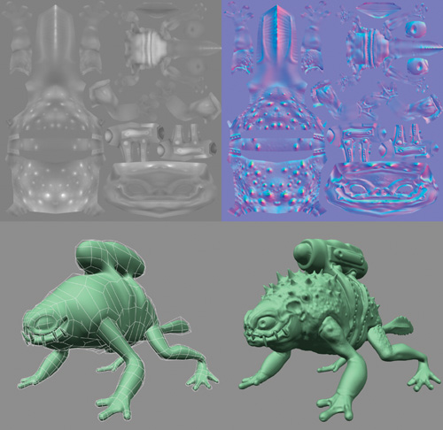
Figure 7-10 An Example of Displacement Mapping
7.3 Conclusion
We have described a method to tessellate subdivision surfaces on the GPU using subdivision with a breadth-first recursion algorithm. We described the shaders necessary to perform flatness testing, to carry out the subdivision, and to compute the limit surface attributes. We also explained how to modify the shaders to add displacement-mapping support for increasing the geometric detail of subdivision surface models.
7.4 References
Catmull, E., and J. Clark. 1978. "Recursively Generated B-Spline Surfaces on Arbitrary Topology Meshes." Computer Aided Design 10(6), pp. 350–355.
DeRose, T., M. Kass, and T. Truong. 1998. "Subdivision Surfaces in Character Animation." In Computer Graphics (Proceedings of SIGGRAPH 98), pp. 85–94.
Halstead, M., M. Kass, and T. DeRose. 1993. "Efficient, Fair Interpolation Using Catmull-Clark Surfaces." In Computer Graphics (Proceedings of SIGGRAPH 93), pp. 35–44.
Copyright
Many of the designations used by manufacturers and sellers to distinguish their products are claimed as trademarks. Where those designations appear in this book, and Addison-Wesley was aware of a trademark claim, the designations have been printed with initial capital letters or in all capitals.
The authors and publisher have taken care in the preparation of this book, but make no expressed or implied warranty of any kind and assume no responsibility for errors or omissions. No liability is assumed for incidental or consequential damages in connection with or arising out of the use of the information or programs contained herein.
NVIDIA makes no warranty or representation that the techniques described herein are free from any Intellectual Property claims. The reader assumes all risk of any such claims based on his or her use of these techniques.
The publisher offers excellent discounts on this book when ordered in quantity for bulk purchases or special sales, which may include electronic versions and/or custom covers and content particular to your business, training goals, marketing focus, and branding interests. For more information, please contact:
U.S. Corporate and Government Sales
(800) 382-3419
corpsales@pearsontechgroup.com
For sales outside of the U.S., please contact:
International Sales
international@pearsoned.com
Visit Addison-Wesley on the Web: www.awprofessional.com
Library of Congress Cataloging-in-Publication Data
GPU gems 2 : programming techniques for high-performance graphics and general-purpose
computation / edited by Matt Pharr ; Randima Fernando, series editor.
p. cm.
Includes bibliographical references and index.
ISBN 0-321-33559-7 (hardcover : alk. paper)
1. Computer graphics. 2. Real-time programming. I. Pharr, Matt. II. Fernando, Randima.
T385.G688 2005
006.66—dc22
2004030181
GeForce™ and NVIDIA Quadro® are trademarks or registered trademarks of NVIDIA Corporation.
Nalu, Timbury, and Clear Sailing images © 2004 NVIDIA Corporation.
mental images and mental ray are trademarks or registered trademarks of mental images, GmbH.
Copyright © 2005 by NVIDIA Corporation.
All rights reserved. No part of this publication may be reproduced, stored in a retrieval system, or transmitted, in any form, or by any means, electronic, mechanical, photocopying, recording, or otherwise, without the prior consent of the publisher. Printed in the United States of America. Published simultaneously in Canada.
For information on obtaining permission for use of material from this work, please submit a written request to:
Pearson Education, Inc.
Rights and Contracts Department
One Lake Street
Upper Saddle River, NJ 07458
Text printed in the United States on recycled paper at Quebecor World Taunton in Taunton, Massachusetts.
Second printing, April 2005
Dedication
To everyone striving to make today's best computer graphics look primitive tomorrow
- Copyright
- Inside Back Cover
- Inside Front Cover
- Part I: Geometric Complexity
-
- Chapter 1. Toward Photorealism in Virtual Botany
- Chapter 2. Terrain Rendering Using GPU-Based Geometry Clipmaps
- Chapter 3. Inside Geometry Instancing
- Chapter 4. Segment Buffering
- Chapter 5. Optimizing Resource Management with Multistreaming
- Chapter 6. Hardware Occlusion Queries Made Useful
- Chapter 7. Adaptive Tessellation of Subdivision Surfaces with Displacement Mapping
- Chapter 8. Per-Pixel Displacement Mapping with Distance Functions
- Part II: Shading, Lighting, and Shadows
-
- Chapter 9. Deferred Shading in S.T.A.L.K.E.R.
- Chapter 10. Real-Time Computation of Dynamic Irradiance Environment Maps
- Chapter 11. Approximate Bidirectional Texture Functions
- Chapter 12. Tile-Based Texture Mapping
- Chapter 13. Implementing the mental images Phenomena Renderer on the GPU
- Chapter 14. Dynamic Ambient Occlusion and Indirect Lighting
- Chapter 15. Blueprint Rendering and "Sketchy Drawings"
- Chapter 16. Accurate Atmospheric Scattering
- Chapter 17. Efficient Soft-Edged Shadows Using Pixel Shader Branching
- Chapter 18. Using Vertex Texture Displacement for Realistic Water Rendering
- Chapter 19. Generic Refraction Simulation
- Part III: High-Quality Rendering
-
- Chapter 20. Fast Third-Order Texture Filtering
- Chapter 21. High-Quality Antialiased Rasterization
- Chapter 22. Fast Prefiltered Lines
- Chapter 23. Hair Animation and Rendering in the Nalu Demo
- Chapter 24. Using Lookup Tables to Accelerate Color Transformations
- Chapter 25. GPU Image Processing in Apple's Motion
- Chapter 26. Implementing Improved Perlin Noise
- Chapter 27. Advanced High-Quality Filtering
- Chapter 28. Mipmap-Level Measurement
- Part IV: General-Purpose Computation on GPUS: A Primer
-
- Chapter 29. Streaming Architectures and Technology Trends
- Chapter 30. The GeForce 6 Series GPU Architecture
- Chapter 31. Mapping Computational Concepts to GPUs
- Chapter 32. Taking the Plunge into GPU Computing
- Chapter 33. Implementing Efficient Parallel Data Structures on GPUs
- Chapter 34. GPU Flow-Control Idioms
- Chapter 35. GPU Program Optimization
- Chapter 36. Stream Reduction Operations for GPGPU Applications
- Part V: Image-Oriented Computing
-
- Chapter 37. Octree Textures on the GPU
- Chapter 38. High-Quality Global Illumination Rendering Using Rasterization
- Chapter 39. Global Illumination Using Progressive Refinement Radiosity
- Chapter 40. Computer Vision on the GPU
- Chapter 41. Deferred Filtering: Rendering from Difficult Data Formats
- Chapter 42. Conservative Rasterization
- Part VI: Simulation and Numerical Algorithms
-
- Chapter 43. GPU Computing for Protein Structure Prediction
- Chapter 44. A GPU Framework for Solving Systems of Linear Equations
- Chapter 45. Options Pricing on the GPU
- Chapter 46. Improved GPU Sorting
- Chapter 47. Flow Simulation with Complex Boundaries
- Chapter 48. Medical Image Reconstruction with the FFT