
GPU Gems 2
GPU Gems 2 is now available, right here, online. You can purchase a beautifully printed version of this book, and others in the series, at a 30% discount courtesy of InformIT and Addison-Wesley.
The CD content, including demos and content, is available on the web and for download.
Chapter 32. Taking the Plunge into GPU Computing
Ian Buck
Stanford University
This and many other chapters in this book demonstrate how we can use GPUs as general computing engines, but it is important to remember that GPUs are primarily designed for interactive rendering, not computation. As a result, you can run into some stumbling blocks when trying to use the GPU as a computing engine. There are significant differences between the GPU and the CPU regarding both capabilities and performance, ranging from memory bandwidth and floating-point number representation to indirect memory access. Because our goal in porting applications to the GPU is to outperform the CPU implementations, it is important to understand these differences and structure our computation optimally for the GPU. In this chapter, we cover some of these differences and show how to write fast and efficient GPU-based applications.
32.1 Choosing a Fast Algorithm
Given that the GPU is primarily designed for rendering, the memory and compute units are optimized for shading rather than general-purpose computing such as signal processing, complex linear algebra, ray tracing, or whatever we might want to cram into the shader pipeline. In this section, we examine some of the performance characteristics of GPUs, contrasting them with CPUs. Understanding these characteristics can help us decide whether a given algorithm can capitalize on the capabilities of the GPU and, if so, how best to structure the computation for the GPU.
32.1.1 Locality, Locality, Locality
Getting good memory performance on CPUs is always about the locality of the references. The same is true for GPUs, but with several important variances. Figure 32-1 shows the performance of reading single-component floating-point texture data on the GeForce 6800 Ultra memory system compared to a 3.0 GHz Pentium 4 with three different access patterns: cached (reading the same memory location repeatedly), sequential, and random. It is clear that the GPU has much higher sequential memory access performance than the CPU. This is not surprising, considering that one of the key tasks of GPUs is filling regions of memory with contiguous texture data. From a computation standpoint, however, to get peak memory performance, computation must be structured around sequential memory accesses or else suffer a huge performance penalty with random memory reads. This is good news for accelerating linear algebra operations such as adding two large vectors, where data is naturally accessed sequentially. However, algorithms that do a lot of pointer chasing are going to suffer from poor random-access performance.
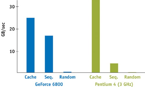
Figure 32-1 Comparing Memory Performance of the GPU and CPU
Another important distinction in memory performance between the GPU and the CPU is the role of the cache. Unlike the cache on the CPU, the GPU texture cache exists primarily to accelerate texture filtering. As a result, GPU caches need to be only as large as the size of the filter kernel for the texture sampler (typically only a few texels), which is too small to be useful for general-purpose computation. GPU cache formats are also optimized for locality in two dimensions, which is not always desirable. This is in contrast to the Pentium 4 cache, which operates at a much higher clock rate and contains megabytes of data. In addition, the Pentium 4 is able to cache both read and write memory operations, while the GPU cache is designed for read-only texture data. Any data written to memory (that is, the frame buffer) is not cached but written out to memory.
What does this mean for general-purpose computation on GPUs? The read-write CPU cache permits programmers to optimize algorithms to operate primarily out of the cache. For example, if your application data set is relatively small, it may fit entirely inside the Pentium 4 cache. Even with larger data sets, an application writer can "block" the computation to ensure that most reads and writes occur in the cache. In contrast, the limited size and read-only nature of the GPU cache puts it at a significant disadvantage. Therefore, an application that is more limited by sequential or random read bandwidth, such as adding two large vectors, will see much more significant performance improvements when ported to the GPU. The vector addition example sequentially reads and writes large vectors with no reuse of the data—an optimal access pattern on the GPU.
32.1.2 Letting Computation Rule
Memory access patterns are not the only determining characteristic in establishing whether an algorithm will run faster on a GPU versus a CPU. Certainly, if an application is dominated by computation, it does not matter much how we access memory. The rate of computation is where GPUs clearly outperform CPUs. Today's GPUs offer more than 60 gigaflops (billions of floating-point operations per second, or Gflops) of computing power in the fragment program hardware alone. Compare this to the Pentium 4 processor, which is limited to only 12 Gflops. [1] Therefore, with enough computation in GPU programs, any differences in memory performance should be unnoticeable.
But how much computation is necessary to avoid becoming limited by memory performance? To answer that question, we need to first review how memory accesses behave on the GPU. When we issue a texture fetch instruction, the memory read is serviced by the texture subsystem, which will likely have to fetch the texel from off-chip memory. To hide the time, or latency, of the texture fetch, the GPU begins work on the next fragment to be shaded after issuing the texel read request. When the texture data returns, the GPU suspends work on the next fragment and returns to continue shading the original fragment. Therefore, if we want to be limited by the computing performance of the GPU and not by the memory, our programs need to contain enough arithmetic instructions to cover the latency of any texture fetches we perform.
As explained in Section 29.1.2 of Chapter 29, "Streaming Architectures and Technology Trends," the number of floating-point operations that GPUs can perform per value read from memory has increased over the past few years and is currently at a factor of seven to ten. From this discrepancy, we can make some conclusions regarding the kinds of GPU-based applications that are likely to outperform their CPU counterparts. To avoid being limited by the memory system, we must examine the ratio of arithmetic and memory operations for a given algorithm. This ratio is called the arithmetic intensity of the algorithm. If an algorithm has high arithmetic intensity, it performs many more arithmetic operations than memory operations. Because today's GPUs have five or more times more computing performance than CPUs, applications with high arithmetic intensity are likely to perform well on GPUs. Furthermore, we are more likely to be able to hide the costs of any memory fetch operations with arithmetic instructions.
32.1.3 Considering Download and Readback
One final performance consideration when using the GPU as a computing platform is the issue of download and readback. Before we even start computing on the GPU, we need to transfer our initial data down to the graphics card. Likewise, if the results of the computation are needed by the CPU, we need to read the data back from the GPU. Performing the computation on the CPU does not require these extra operations. When comparing against the CPU, we must consider the performance impact of downloading and reading back data.
Consider the example of adding two large vectors on the GPU. Executing a fragment program that simply fetches two floating-point values, adds them, and writes the result will certainly run faster than a CPU implementation, for reasons explained earlier. However, if we add the cost of downloading the vector data and reading back the results to the CPU, we are much better off simply performing the vector add on the CPU. Peak texture download and readback rates for today's PCI Express graphics cards max out around 3.2 GB/sec. A 3.0 GHz Pentium 4 can add two large vectors at a rate of approximately 700 megaflops (millions of floating-point operations per second, or Mflops). [2] So before we could even download both of the vectors to the GPU, the CPU could have completed the vector addition.
To avoid this penalty, we need to amortize the cost of the download and readback of our data. For simulation applications, this is less of a problem, because most such algorithms iterate over the data many times before returning. However, if you plan to use the GPU to speed up linear algebra operators (such as vector add), make sure you are doing enough operations on the data to cover the additional cost of download and readback.
One further consideration is the different pixel formats. Not all texture and frame-buffer formats operate at the same speed. In some cases, the graphics driver may have to use the CPU to convert from user data provided as RGBA to the native GPU format, which might be BGRA. This can significantly affect download and readback performance. Native formats vary between vendors and different GPUs. It is best to experiment with a variety of formats to find the one that is fastest.
32.2 Understanding Floating Point
Today's GPUs perform all their computation using floating-point arithmetic. While desktop CPUs generally support a single floating-point standard, GPU vendors have implemented a variety of floating-point formats. Understanding the differences between these formats can help you both understand whether your application can produce accurate results and avoid some of the more common floating-point arithmetic mistakes, which can be more treacherous when using GPUs compared to CPUs.
First, let's review floating-point representation. A floating-point number is represented by the following expression:
|
sign x 1.matissa x 2(exponent-bias). |
Consider representing the number 143.5, which corresponds to 1.435 x 10² in scientific notation. The scientific binary representation is 1.00011111 x 2111. Thus the mantissa is set to 00011111 (the leading 1 is implied), and the exponent is stored biased by 127 (set by the particular floating-point format standard), which corresponds to 10000110. Different floating-point formats have differing numbers of bits dedicated to the mantissa and the exponent. For example, in the IEEE 754 standard used by most CPUs, a 32-bit float value consists of 1 sign bit, an 8-bit exponent, and a 23-bit mantissa. The number of bits available in the mantissa and exponent determines how accurately we can represent numbers. For IEEE 754, 143.5 is represented exactly; however 143.98375329 is rounded to 143.98375, because there are only 23 bits available for the mantissa. The GPU floating-point formats available today are the following:
- NVIDIA fp32: 23-bit mantissa, 8-bit exponent
- ATI fp24: 16-bit mantissa, 7-bit exponent
- NVIDIA fp16: 10-bit mantissa, 5-bit exponent
What does this mean for GPU-based applications? First, the NVIDIA fp32 format mimics the CPU, so calculations performed in that format should be accurate to approximately the seventh significant digit, which is the limit of the 23-bit mantissa. In contrast, ATI fp24 should be accurate to the fifth significant digit, while the NVIDIA fp16 format is accurate to the third digit. Although such lower precisions are perfectly reasonable for shading computations where the exact color value is not critical, the errors introduced from these formats can grossly affect numerical applications. Table 32-1 illustrates how accurately we can represent the number 143.98375329 with the different formats.
Table 32-1. Comparing the Accuracy of Floating-Point Formats
|
Number to represent: 143.98375329 |
||
|
Format |
Result |
Error |
|
NVIDIA fp32 |
143.98375 |
0.00000329 (2 x 10⁻⁶%) |
|
ATI fp24 |
143.98242 |
0.00133329 (9 x 10⁻⁴%) |
|
NVIDIA fp16 |
143.875 |
0.10875329 (7 x 10⁻²%) |
32.2.1 Address Calculation
One particularly nasty consequence of this limited floating-point precision occurs when dealing with address calculations. Consider the case where we are computing addresses into a large 1D array that we'll store in a 2D texture. When computing a 1D address, it may be possible to end up with unaddressable elements of the array, due to the limited precision of the floating-point arithmetic. For example, if we are using an NVIDIA fp16 float, we cannot address element 3079, because the closest representable numbers with a 10-bit mantissa are 3078 and 3080. These off-by-one addressing bugs can be difficult to track down, because not all calculations will generate them. Even with 24-bit floats, it is not possible to address all of the pixels in a large 2D texture with a 1D address. Table 32-2 specifies the largest possible counting number that can be represented in each of the different formats before integer values start to be skipped.
Table 32-2. Comparing the Last Representable Integer Before Values Start to Be Skipped
|
Format |
Largest Number |
|
NVIDIA fp32 |
16,777,216 |
|
ATI fp24 |
131,072 |
|
NVIDIA fp16 |
2,048 |
As future GPUs begin to provide integer arithmetic, address calculation should become less of a problem. Until then, be aware of the floating-point precision you are using in your application, particularly when relying on floating-point values for memory addressing.
32.3 Implementing Scatter
One of the first things GPU programmers discover when using the GPU for general-purpose computation is the GPU's inability to perform a scatter operation in the fragment program. A scatter operation, also called an indirect write, is any memory write operation from a computed address. For example, the C code a[i] = x is a scatter operation in which we are "scattering" the value x into the array a from a computed address i. Scatter operations are extremely common in even the most basic algorithms. Examples include quicksort, hashing, histograms, or any algorithm that must write to memory from a computed address.
To see why scatters are hard to implement in a fragment program, let's look at the opposite of a scatter operation: gather. A gather is an indirect read operation, such as x = a[i]. Implementing gather inside a fragment program is straightforward, because it corresponds to a dependent texture read. For example, a is a texture, i is any computed value, and a[i] is a simple texture fetch instruction. Implementing scatter (a[i] = x) in a fragment program is not so simple, because there is no texture write instruction. In fact, the only memory writes we can perform in the GPU are at the precomputed fragment address, which cannot be changed by a fragment program. Each fragment writes to a fixed position in the frame buffer. In this section, we discuss some ways to get around this limitation of GPUs for applications that need to scatter data.
32.3.1 Converting to Gather
In some cases, it is possible to convert a scatter operation into a gather operation. To illustrate this, let's consider the example of simulating a spring-mass system on the GPU.
Figure 32-2 illustrates a simple mass-spring system in which we loop over each spring, compute the force exerted by the spring, and add the force contribution to the masses connected to the spring. The problem with implementing this algorithm on the GPU is that the spring force is scattered to the mass_force array. This scatter cannot be performed inside the fragment program.
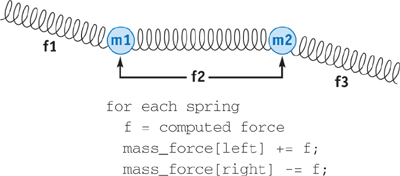
Figure 32-2 A Simple Spring-Mass System, Updated with a Scatter
We can convert the scatter into a gather by performing another pass over the array into which we were previously scattering. As shown in Figure 32-3, instead of scattering the forces, we first output the spring forces to memory. With a second pass, we loop over all of the masses and gather the force values that affect that mass. [3] In general, this technique works wherever the connectivity is static. Because the spring connectivity is not changing during our simulation, we know exactly which element in the forces array we need to gather for each mass.
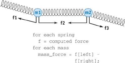
Figure 32-3 New Mass-Spring System with Only Gather Operations
32.3.2 Address Sorting
But what if our scatter address is not fixed? For example, let's assume we are implementing a particle simulation in which we have divided space into a grid of rectangular voxels. We wish to compute the net particle velocity for each voxel of the space. This type of operation is common when working with level sets. Figure 32-4 shows a typical implementation.
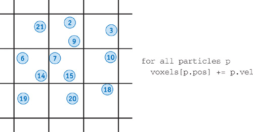
Figure 32-4 Computing the Net Particle Velocity in a Voxel
Here the address we are using for the scatter is not fixed, because the particles are moving from voxel to voxel in each time step of our simulation. We cannot convert this scatter into a gather directly because we don't know where to fetch our scatter data until runtime.
We can still convert these scatter operations into gathers using a technique called address sorting. The algorithm is similar to the earlier example except instead of simply outputting the data to scatter, we also output the scatter address with the data. We can then sort the data address pairs based on the address. This places all of the data to be scattered in contiguous array locations. Finally, we loop over each element of the array into which we want to scatter, using a binary search to fetch the data to scatter. See Figure 32-5.
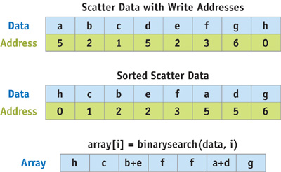
Figure 32-5 Converting Scatters to Gathers with Address Sorting
Using address sorting to convert scatters to gathers is a fairly extensive multipass solution, but it may be the only option if your scatter addresses are not fixed in advance. Exactly how to implement sorting and searching on the GPU is explained in Buck and Purcell 2004, as well as in Chapter 46 of this book, "Improved GPU Sorting."
32.3.3 Rendering Points
Although fragment programs cannot change the address to which they are writing, vertex programs can by their very nature specify where to render in the output image. We can therefore use a vertex program to perform our scatter operation. This technique is fairly straightforward. The application simply issues points to render and the vertex program fetches from texture the scatter address and assigns it to the point's destination address with the appropriate scatter data. If the GPU does not support vertex textures, we can use the vertex and pixel buffer object extensions to remap texture data into a vertex array. The downside to this approach is that rendering points does not make very efficient use of the rasterization hardware. Also, you will have to be conscious of collisions in the scatter addresses (that is, when two points end up in the same position). Some simple ways to resolve collisions are either to use the z-buffer to prioritize them or to use blending operations to combine the values.
In summary, if you need to perform a scatter operation, you should convert the scatter into gather operations wherever you have fixed scatter addresses. If your scatter addresses are not fixed, you can use either address sorting or point rendering. Deciding which will be faster may differ from GPU to GPU; however, in general, if you are going to do very few scatters into a large region of memory, consider rendering points. The time it takes to scatter data with point rendering is a function of only the number of values to scatter. If you are scattering lots of data, it may be better to use the address sorting method to avoid reading data back to the CPU or being limited by the rate at which the GPU can render points.
32.4 Conclusion
In this chapter, we have touched on some of the challenges programmers discover when transitioning from CPU-based to GPU-based computing. To outperform the CPU, we need to understand GPU performance strengths, specifically favoring algorithms with sequential memory access and a good ratio of computation to memory operations. In addition, we have discussed some of the different types of floating-point formats available on GPUs and how they can affect the correctness of a program. Finally, we've shown how to work around the GPU's limited support for scatter operations. As you discover how the GPU can be used to accelerate your own algorithms, we hope the strategies described in this chapter will help you improve your application through efficient GPU-based computing.
32.5 References
Buck, Ian, and Purcell, Tim. 2004. "A Toolkit for Computation on GPUs." In GPU Gems, edited by Randima Fernando, pp. 621–636. Addison-Wesley.
Fatahalian, Kayvon, Jeremy Sugerman, and Pat Hanrahan. 2004. "Understanding the Efficiency of GPU Algorithms for Matrix-Matrix Multiplication." Proceedings of Graphics Hardware.
Goldberg, David. 1991. "What Every Computer Scientist Should Know About Floating Point Arithmetic. ACM Computing Surveys 23(1), pp. 5–48.
IEEE Standards Committee 754. 1987. "IEEE Standard for Binary Floating-Point Arithmetic, ANSI/IEEE Standard 754-1985." Reprinted in SIGPLAN Notices 22(2), pp. 9–25.
NVIDIA fp16 specification. Available online at http://www.nvidia.com/dev_content/nvopenglspecs/GL_NV_half_float.txt
Copyright
Many of the designations used by manufacturers and sellers to distinguish their products are claimed as trademarks. Where those designations appear in this book, and Addison-Wesley was aware of a trademark claim, the designations have been printed with initial capital letters or in all capitals.
The authors and publisher have taken care in the preparation of this book, but make no expressed or implied warranty of any kind and assume no responsibility for errors or omissions. No liability is assumed for incidental or consequential damages in connection with or arising out of the use of the information or programs contained herein.
NVIDIA makes no warranty or representation that the techniques described herein are free from any Intellectual Property claims. The reader assumes all risk of any such claims based on his or her use of these techniques.
The publisher offers excellent discounts on this book when ordered in quantity for bulk purchases or special sales, which may include electronic versions and/or custom covers and content particular to your business, training goals, marketing focus, and branding interests. For more information, please contact:
U.S. Corporate and Government Sales
(800) 382-3419
corpsales@pearsontechgroup.com
For sales outside of the U.S., please contact:
International Sales
international@pearsoned.com
Visit Addison-Wesley on the Web: www.awprofessional.com
Library of Congress Cataloging-in-Publication Data
GPU gems 2 : programming techniques for high-performance graphics and general-purpose
computation / edited by Matt Pharr ; Randima Fernando, series editor.
p. cm.
Includes bibliographical references and index.
ISBN 0-321-33559-7 (hardcover : alk. paper)
1. Computer graphics. 2. Real-time programming. I. Pharr, Matt. II. Fernando, Randima.
T385.G688 2005
006.66—dc22
2004030181
GeForce™ and NVIDIA Quadro® are trademarks or registered trademarks of NVIDIA Corporation.
Nalu, Timbury, and Clear Sailing images © 2004 NVIDIA Corporation.
mental images and mental ray are trademarks or registered trademarks of mental images, GmbH.
Copyright © 2005 by NVIDIA Corporation.
All rights reserved. No part of this publication may be reproduced, stored in a retrieval system, or transmitted, in any form, or by any means, electronic, mechanical, photocopying, recording, or otherwise, without the prior consent of the publisher. Printed in the United States of America. Published simultaneously in Canada.
For information on obtaining permission for use of material from this work, please submit a written request to:
Pearson Education, Inc.
Rights and Contracts Department
One Lake Street
Upper Saddle River, NJ 07458
Text printed in the United States on recycled paper at Quebecor World Taunton in Taunton, Massachusetts.
Second printing, April 2005
Dedication
To everyone striving to make today's best computer graphics look primitive tomorrow
- Copyright
- Inside Back Cover
- Inside Front Cover
- Part I: Geometric Complexity
-
- Chapter 1. Toward Photorealism in Virtual Botany
- Chapter 2. Terrain Rendering Using GPU-Based Geometry Clipmaps
- Chapter 3. Inside Geometry Instancing
- Chapter 4. Segment Buffering
- Chapter 5. Optimizing Resource Management with Multistreaming
- Chapter 6. Hardware Occlusion Queries Made Useful
- Chapter 7. Adaptive Tessellation of Subdivision Surfaces with Displacement Mapping
- Chapter 8. Per-Pixel Displacement Mapping with Distance Functions
- Part II: Shading, Lighting, and Shadows
-
- Chapter 9. Deferred Shading in S.T.A.L.K.E.R.
- Chapter 10. Real-Time Computation of Dynamic Irradiance Environment Maps
- Chapter 11. Approximate Bidirectional Texture Functions
- Chapter 12. Tile-Based Texture Mapping
- Chapter 13. Implementing the mental images Phenomena Renderer on the GPU
- Chapter 14. Dynamic Ambient Occlusion and Indirect Lighting
- Chapter 15. Blueprint Rendering and "Sketchy Drawings"
- Chapter 16. Accurate Atmospheric Scattering
- Chapter 17. Efficient Soft-Edged Shadows Using Pixel Shader Branching
- Chapter 18. Using Vertex Texture Displacement for Realistic Water Rendering
- Chapter 19. Generic Refraction Simulation
- Part III: High-Quality Rendering
-
- Chapter 20. Fast Third-Order Texture Filtering
- Chapter 21. High-Quality Antialiased Rasterization
- Chapter 22. Fast Prefiltered Lines
- Chapter 23. Hair Animation and Rendering in the Nalu Demo
- Chapter 24. Using Lookup Tables to Accelerate Color Transformations
- Chapter 25. GPU Image Processing in Apple's Motion
- Chapter 26. Implementing Improved Perlin Noise
- Chapter 27. Advanced High-Quality Filtering
- Chapter 28. Mipmap-Level Measurement
- Part IV: General-Purpose Computation on GPUS: A Primer
-
- Chapter 29. Streaming Architectures and Technology Trends
- Chapter 30. The GeForce 6 Series GPU Architecture
- Chapter 31. Mapping Computational Concepts to GPUs
- Chapter 32. Taking the Plunge into GPU Computing
- Chapter 33. Implementing Efficient Parallel Data Structures on GPUs
- Chapter 34. GPU Flow-Control Idioms
- Chapter 35. GPU Program Optimization
- Chapter 36. Stream Reduction Operations for GPGPU Applications
- Part V: Image-Oriented Computing
-
- Chapter 37. Octree Textures on the GPU
- Chapter 38. High-Quality Global Illumination Rendering Using Rasterization
- Chapter 39. Global Illumination Using Progressive Refinement Radiosity
- Chapter 40. Computer Vision on the GPU
- Chapter 41. Deferred Filtering: Rendering from Difficult Data Formats
- Chapter 42. Conservative Rasterization
- Part VI: Simulation and Numerical Algorithms
-
- Chapter 43. GPU Computing for Protein Structure Prediction
- Chapter 44. A GPU Framework for Solving Systems of Linear Equations
- Chapter 45. Options Pricing on the GPU
- Chapter 46. Improved GPU Sorting
- Chapter 47. Flow Simulation with Complex Boundaries
- Chapter 48. Medical Image Reconstruction with the FFT