
GPU Gems 2
GPU Gems 2 is now available, right here, online. You can purchase a beautifully printed version of this book, and others in the series, at a 30% discount courtesy of InformIT and Addison-Wesley.
The CD content, including demos and content, is available on the web and for download.
Chapter 45. Options Pricing on the GPU
Craig Kolb
NVIDIA Corporation
Matt Pharr
NVIDIA Corporation
In the past three decades, options and other derivatives have become increasingly important financial tools. Options are commonly used to hedge the risk associated with investing in securities, and to take advantage of pricing anomalies in the market via arbitrage.
A key requirement for utilizing options is calculating their fair value. Finding ways of efficiently solving this pricing problem has been an active field of research for more than thirty years, and it continues to be a focus of modern financial engineering. As more computation has been applied to finance-related problems, finding efficient ways to implement these algorithms on modern architectures has become more important.
This chapter describes how options can be priced efficiently using the GPU. We perform our evaluations using two different pricing models: the Black-Scholes model and lattice models. Both of these approaches map well to the GPU, and both are substantially faster on the GPU than on modern CPUs. Although both also have straightforward mappings to the GPU, implementing lattice models requires additional work because of interdependencies in the calculations.
45.1 What Are Options?
Options belong to the family of investment tools known as derivatives. Traditional investment instruments, such as real estate or stocks, have inherent value. Options, on the other hand, derive their value from another investment instrument, known as the underlying asset. The underlying asset is typically stock or another form of security.
Options come in several varieties. A call option contract gives the purchaser (or holder) the right, but not the obligation, to buy the underlying asset for a particular, predetermined price at some future date. The predetermined price is known as the strike price, and the future date is termed the expiration date. Similarly, a put gives the holder the option of selling the underlying asset for a predetermined price on the expiration date.
For example, consider a call option written on the stock of the XYZ Corporation. Imagine that this contract guaranteed that you could buy 100 shares of XYZ's stock at a price of $100 six months from today. If the stock were trading for less than $100 on the date of expiration, it would make little sense to exercise the option—you could buy the stock for less money on the open market, after all. In this case, you would simply let the option expire, worthless. On the other hand, if XYZ were trading for, say, $120 per share on the expiration date, you would exercise the option to buy the shares at $100 each. If you then sold the shares immediately, you would profit $20 a share, minus whatever you had paid for the option.
As just illustrated, both the strike price, X, and the price of the underlying asset at the expiration date strongly influence the future value of the option, and thus how much you should pay for it today. Under certain simplifying assumptions, we can statistically model the asset's future price fluctuations using its current price, S, and its volatility, v, which describes how widely the price changes over time.
A number of additional factors influence how much you'd likely be willing to pay for an option:
- The time to the expiration date, T. Longer terms imply a wider range of possible values for the underlying asset on the expiration date, and thus more uncertainty about the value of the option when it expires.
- The riskless rate of return, r. Even if the option made you a profit of P
dollars six months from now, the value of those P dollars to you today is less than P. If a
bond or other "riskless" investment paid interest at a continually compounded annual rate of r, you
could simply invest P x e -r(6/12) dollars in the bond today, and you
would be guaranteed the same P dollars six months from now. As such, the value of an asset at some
future time 0 < t
 T
must be discounted by multiplying it by e -rt in order to determine its
effective value today.
T
must be discounted by multiplying it by e -rt in order to determine its
effective value today.
- Exercise restrictions. So far, we have discussed only so-called European options, which may be exercised only on the day the option expires. Other types of options with different exercise restrictions also exist. In particular, American options may be exercised at any time up to and including the expiration date. This added flexibility means that an American option will be priced at least as high as the corresponding European option.
Other factors, such as dividend payouts, can also enter into the picture. For this chapter, however, we will limit ourselves to the preceding considerations.
The rest of this chapter describes two standard methods of pricing options and how they are traditionally implemented on the CPU. We show how these methods can be implemented on the GPU with greater throughput, as measured by the number of options priced per second.
We omit the majority of the mathematical details in the discussion that follows. See Hull 2002 for extensive background material, including supporting theory, derivations, and assumptions used in these pricing models.
45.2 The Black-Scholes Model
In 1973, Fischer Black and Myron Scholes famously derived an analytical means of computing the price of European options (Black and Scholes 1973). For this work, Scholes was awarded the Nobel Prize for economics in 1997. (Black had passed away before the prize was awarded.)
The Black-Scholes equation is a differential equation that describes how, under a certain set of assumptions, the value of an option changes as the price of the underlying asset changes. More precisely, it is a stochastic differential equation; it includes a random-walk term—which models the random fluctuation of the price of the underlying asset over time—in addition to a deterministic term. This random term necessitates using slightly different mathematical tools than you'd normally use to solve differential equations; see the references for details.
The Black-Scholes equation implies that the value of a European call option, V, may be computed as:
|
V = S x CND(d1 ) - Xe-rT x CND(d2 ), |
where
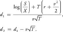
(The formula for a put option is similar.) The cumulative normal distribution function, CND(x), gives the probability that a normally distributed random variable will have a value less than x. There is no closed-form expression for this function, and as such it must be evaluated numerically. It is typically approximated using a polynomial function, as we do here.
We use the GPGPU framework described in Chapter 31 of this book, "Mapping Computational Concepts to GPUs," together with the Cg code in Listing 45-1, to price options in parallel on the GPU. We first initialize four 2D arrays of data with the exercise price, asset price, time to expiration, and asset volatility corresponding to each option, with the input data for a particular option residing at the same location in each array. It is then a simple matter to price all of the options in parallel by running the fragment program at every pixel. For our tests, we assumed that the riskless rate of return for all options was constant and thus could be given via a uniform parameter to the Cg program. For some applications, it may also be useful to vary this value, a straightforward change to the program. The implementation of the cumulative normal distribution function, CND(), is shown later in Listing 45-2.
Example 45-1. Implementing the Black-Scholes Model in Cg
float BlackScholesCall(float S, float X, float T, float r, float v)
{
  float d1 = (log(S / X) + (r + v * v * .5f) * T) / (v * sqrt(T));
  float d2 = d1 - v * sqrt(T);
  return S * CND(d1) - X * exp(-r * T) * CND(d2);
}
Pricing a given option using this method thus depends on five input parameters, requires a relatively large amount of floating-point calculation, and produces a single float-point value. The result is a computation with very high arithmetic intensity, making it extremely well suited for running on the GPU, as can be seen in Figure 45-1.
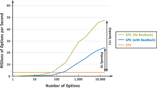
Figure 45-1 GPU vs. CPU Performance of Black-Scholes Option Pricing
Listing 45-2 shows that, rather than directly evaluate the polynomial—for example, using Horner's rule—a more efficient approach for the GPU is to take advantage of its four-way vector hardware, precompute the powers of K, and use the dot() function to quickly compute an inner product with appropriate constants.
Interestingly enough, the PCI Express bus has the potential to be the bottleneck for a GPU implementation of this model: assuming ideal PCI Express performance of 4 GB/sec of bandwidth, it is possible to transfer 1 billion 4-byte floating-point values to and from the GPU each second. For our test program, 4 of the input parameters were varying, which means that it is possible to feed the GPU enough data to do roughly 250 million Black-Scholes computations per second (4 GB/sec divided by 4 values times 4 bytes per float value). The Black-Scholes implementation here compiles to approximately 50 floating-point operations. Therefore, any GPU that is capable of more than 10 Gflops of arithmetic computation will be limited by the rate at which data can be sent to the GPU (recall that current GPUs are capable of hundreds of Gflops of computation).
Example 45-2. Implementing the Cumulative Normal Distribution Function
float CND(float X)
{
  float L = abs(X);
  // Set up float4 so that K.x = K, K.y = K^2, K.z = K^3, K.w = K^4
  float4 K;
  K.x = 1.0 / (1.0 + 0.2316419 * L);
  K.y = K.x * K.x;
  K.zw = K.xy * K.yy;
  // compute K, K^2, K^3, and K^4 terms, reordered for efficient
  // vectorization. Above, we precomputed the K powers; here we'll
  // multiply each one by its corresponding scale and sum up the
  // terms efficiently with the dot() routine.
  //
  // dot(float4(a, b, c, d), float4(e, f, g, h)) efficiently computes
  // the inner product a*e + b*f + c*g + d*h, making much better
  // use of the 4-way vector floating-point hardware than a
  // straightforward implementation would.
  float w =
      dot(float4(0.31938153f, -0.356563782f, 1.781477937f, -1.821255978f), K);
  // and add in the K^5 term on its own
  w += 1.330274429f * K.w * K.x;
  w *= rsqrt(2.f * PI) * exp(-L * L * .5f); // rsqrt() == 1/sqrt()
  if (X > 0)
    w = 1.0 - w;
  return w;
}
In spite of this potential bottleneck, the GPU is still substantially faster than the CPU for our implementation: it is effectively able to run at its peak potential computational rate, subject to PCI Express limitations. For complete applications that need to compute option prices, it is likely that additional computation would be done on the GPU with the Black-Scholes results, which also reduces the impact of PCI Express bandwidth. (In general, the GPU works best as more computation is done on it and there is less communication with the CPU. The PCI Express bandwidth limitation is just a manifestation of the fact that the GPU particularly excels as the ratio of computation to bandwidth increases, as discussed in Chapter 29 of this book, "Streaming Architectures and Technology Trends.")
45.3 Lattice Models
The Black-Scholes equation provides a convenient analytical method of computing the price of European options. However, it is not suitable for pricing American options, which can be exercised at any time prior to the date of expiration. In fact, there is no known closed-form expression that gives the fair price of an American option under the same set of assumptions used by the Black-Scholes equation.
Another family of option pricing models is lattice models. These models use a dynamic programming approach to derive the value of an option at time 0 (that is, now) by starting at time T (that is, the expiration date) and iteratively stepping "backward" toward t = 0 in a discrete number of time steps, N. This approach is versatile and simple to implement, but it can be computationally expensive due to its iterative nature. In this section, we discuss the implementation of the binomial lattice model on the GPU and how it can be used to compute prices of both European and American options.
45.3.1 The Binomial Model
The most commonly used lattice model is the binomial model. The binomial model is so named because it assumes
that if the underlying asset has a price Sk at time step k, its price at step
k + 1 can take on only two possible values, uSk and dS k,
corresponding to an "up" or "down" movement in the price of the stock. Typically, u is calculated by
assuming that during a small time duration dt, the change of the asset value is normally distributed,
with a standard deviation equal to S k v
 .
.
If d is chosen such that u x d = 1, the possible asset prices during the lifetime of the option form a tree, as shown in Figure 45-2. Each path from the root node of the tree to a leaf corresponds to a "walk" of the underlying asset's price over time. The set of nodes at depth k from the root represent the range of possible asset prices at time t = k x dt, where dt = T/N. The leaf nodes, at depth k = N, represent the range of prices the asset might have at the time the option expires.
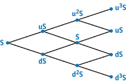
Figure 45-2 Binomial Tree of = 3 Steps, with Associated Asset Prices
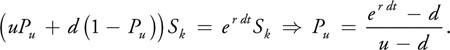
To price the option using the binomial tree, we also compute the pseudo-probability Pu that the asset price will move "up" at any given time. The pseudo-probability of a down movement is simply 1 - Pu . To compute the value of Pu, we assume a risk-neutral world, which implies that the expected return on the underlying asset is equal to r:
Although Pu is not a true probability (that is, it is not the actual probability that the asset price will move up), it is useful to treat it as such, as shown in the following discussion.
45.3.2 Pricing European Options
Given a tree of asset values over time, like the one shown in Figure 45-2, we can calculate an option value at each node of the tree. The value computed for a node at depth k gives the expected value of the option at time t = k x dt, assuming that the underlying asset takes on the range of prices associated with the node's children in the future. Our problem, then, is to compute the value of the option at the root of the tree. We do so by starting at the leaves and working backward toward the root.
Computing the option value at each leaf node i is simple. First we calculate the asset price Si associated with each leaf node directly by raising u to the appropriate power (recall that d = u -1) and multiplying the result by S. Next we compute the corresponding value of the option at each leaf, V i . On the expiration date, a call option is worthless if Si > X; otherwise, it has a value of X - Si . The computation is similar for put options. Using these initial values, we can then calculate the option value for each node at the previous time step. We do so by computing the expected future value of the option using the "probability" of an upward movement, Pu, and the option values associated with the nodes in the "up" and "down" directions, Vi,up and Vi,down . We then discount this future expected value by e-r dt to arrive at the option value corresponding to the node:

We perform this computation for all nodes at a given level of the tree, and then iteratively repeat for the next-highest level, and so on until reaching the root of the tree. The value at the root gives us the value of the option at t = 0: "now". Pseudocode for this algorithm (assuming a European call option) is shown in Listing 45-3. A 1D array, V, is used to iteratively compute option values. At termination, V[0] holds the value of the option at the present time.
Example 45-3. Pseudocode for Pricing a European Put Option Using the Binomial Method
 dt = T/N
u = exp(v * sqrt(dt))
d = 1/u
disc = exp(r * dt)
Pu = (disc - d) / (u - d)
// initialize option value array with values at expiry
for i = 0 to N
Si = S * pow(u, 2 * i - N)
V[i] = max(0, X - Si)
// for each time step
for j = N-1 to 0
// for each node at the current time step
for i = 0 to j
// compute the discounted expected value of the option
V[i] = ((1 - Pu) * V[i] + Pu * V[i + 1])/disc
To adapt the binomial model to run on the GPU, we need to deal with the fact that, unlike Black-Scholes, this calculation is iterative and requires the use of intermediate computed values—the various values of V[i]. One way to parallelize this task for the GPU is to work on a single time step (column) of the binomial tree at a time: one thread is launched for each node of a column of the tree, and it computes the option value for that node. Starting with the rightmost column, the option value at expiry is computed. For the column associated with each previous time step, in turn, option values are computed using the previously computed values for the two child nodes in the manner described earlier. This strategy is illustrated in Figure 45-3. After each thread computes its result, those values are used as input to a new set of threads launched to compute values for the next column to the left. (The general ideas behind this process are related to how reductions are computed on the GPU, as described in Chapter 31 of this book.)
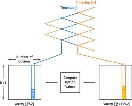
Figure 45-3 Computation Strategy and Data Layout
To increase the parallelism available to the GPU, our implementation simultaneously runs this algorithm for a thousand or so independent options to price at the same time. Thus, the total number of threads running on the GPU at any time is equal to the number of options being priced times the number of tree nodes in the column currently being processed. This additional parallelism is easy to incorporate, and it gives better GPU performance than just parallelizing over a single option-pricing calculation at a time.
We use two fragment programs to price the set of options. The first program computes the initial N + 1 leaf option values (V[0] . . . V[N]) and corresponds to the first for loop in Listing 45-3. The second program is run multiple times to iteratively compute the V[i]s for the interior nodes. The application invokes this program N times, one for each time step (corresponding to the second for loop in Listing 45-3), with each iteration using the previously computed V[i]s to compute the values for the current time step. Each invocation of the program corresponds to the innermost for loop in Listing 45-3; as shown there, at each iteration, the number of computed nodes is reduced by one, leaving us with a single result value corresponding to V[0].
Running the second program involves using the output of one iteration as the input to the next. To do so efficiently, we use a double-buffered pbuffer, which avoids context switching and texture copying overhead. The Cg code for these programs is shown in Listing 45-4, and the pseudocode for driving them is given in Listing 45-5.
Example 45-4. Computing Lattice Model Option Pricing
void init(Stream stockPrice, Stream strikePrice, Stream yearsToMaturity,
          Stream volatility, uniform float riskFreeRate, uniform float numSteps,
          float2 offset
          : DOMAIN0, out float4 result
          : RANGE0)
{
  float deltaT = yearsToMaturity.value(offset.x) / numSteps;
  float u = exp(volatility.value(offset.x) * sqrt(deltaT));
  float price =
      stockPrice.value(offset.x) * pow(u, 2 * (offset.y - 0.5) - numSteps);
  float value = max(strikePrice.value(offset.x) - price, 0);
  result = value;
}
void iterate(Stream Pu, Stream Pd, Stream optval, float2 offset
             : DOMAIN0, float2 offsetplus1
             : DOMAIN1, out float4 result
             : RANGE0)
{
  float val = (Pu.value(offset.x) * optval.value(offsetplus1) +
               Pd.value(offset.x) * optval.value(offset));
  result = val;
}
Example 45-5. Lattice Model Application Pseudocode
 domain = [0, nproblems, 0, N + 1]
Varray[N % 2] = init(Range, S, X, T, v, r, N, domain)
for j = N - 1 to 0
offset = [0, nproblems, 0, j + 1]
offsetplus1 = [0, nproblems, 1, j + 2]
Varray[(j % 2)] = iterate(Pu, Pd, Varray[((j + 1) % 2)], offset,
offsetplus1)
As we increase the number of time steps N, the value computed using the binomial method converges to that computed by the Black-Scholes method. The binomial method is far more computationally expensive than the Black-Scholes method; its asymptotic time complexity is O(N 2), for example, versus Black-Scholes's O(1). However, this computational expense does come with an advantage: unlike Black-Scholes, lattice methods can be adapted for use on a wide variety of options-pricing problems.
For example, we can modify the previous algorithm to price American options. When calculating the expected value of holding the option at each node, we can also compute the value of exercising it immediately. If exercising is more valuable than holding, we set the value of the option at that node to the exercise value, rather than the expected value of holding. In the case of a call option, the value of exercising is X - Si , where Si is the computed price of the asset at node i. A full implementation may be found on the CD that accompanies this book.
As with Black-Scholes, the GPU outperforms the CPU when pricing American options with the binomial approach, as shown in Figure 45-4. As in Figure 45-1, a GeForce 6800 was used for the GPU tests, and an AMD Athlon 64 3200+ was used for the CPU tests.
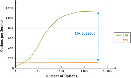
Figure 45-4 GPU vs. CPU Performance of a Binomial Lattice Model with = 1024 Steps
45.4 Conclusion
Both the Black-Scholes model and the lattice model for option pricing are basic building blocks of computational finance. In this chapter, we have shown how the GPU can be used to price options using these models much more efficiently than the CPU. As GPUs continue to become faster more quickly than CPUs, the gap between the two is likely to grow for this application.
Another widely used approach for pricing options is to implement algorithms based on Monte Carlo or quasi-Monte Carlo simulation. These algorithms are also well suited to the GPU, because they rely on running a large number of independent trials and then computing overall estimates based on all of the trials together. The independent trials are trivially parallelizable, and producing the final estimates is a matter of computing reductions. The early-exercise right associated with American options makes it challenging to use Monte Carlo methods to compute their fair value. Finding the means to do so efficiently is an active area of research.
One detail that makes these algorithms slightly more difficult to map to the GPU is the lack of native integer instructions, which are the basis for the pseudorandom number generators needed for Monte Carlo and the low-discrepancy sequences used for quasi-Monte Carlo. This limitation can be sidestepped on current GPUs by generating these numbers on the CPU and downloading them to the GPU. As long as a reasonable amount of computation is done with each random or quasi-random sample, this step isn't a bottleneck.
45.5 References
Black, Fischer, and Myron Scholes. 1973. "The Pricing of Options and Corporate Liabilities." Journal of Political Economy 81(3), pp. 637–654.
Hull, John C. 2002. Options, Futures, and Other Derivatives, 5th ed. Prentice Hall.
Copyright
Many of the designations used by manufacturers and sellers to distinguish their products are claimed as trademarks. Where those designations appear in this book, and Addison-Wesley was aware of a trademark claim, the designations have been printed with initial capital letters or in all capitals.
The authors and publisher have taken care in the preparation of this book, but make no expressed or implied warranty of any kind and assume no responsibility for errors or omissions. No liability is assumed for incidental or consequential damages in connection with or arising out of the use of the information or programs contained herein.
NVIDIA makes no warranty or representation that the techniques described herein are free from any Intellectual Property claims. The reader assumes all risk of any such claims based on his or her use of these techniques.
The publisher offers excellent discounts on this book when ordered in quantity for bulk purchases or special sales, which may include electronic versions and/or custom covers and content particular to your business, training goals, marketing focus, and branding interests. For more information, please contact:
U.S. Corporate and Government Sales
(800) 382-3419
corpsales@pearsontechgroup.com
For sales outside of the U.S., please contact:
International Sales
international@pearsoned.com
Visit Addison-Wesley on the Web: www.awprofessional.com
Library of Congress Cataloging-in-Publication Data
GPU gems 2 : programming techniques for high-performance graphics and general-purpose
computation / edited by Matt Pharr ; Randima Fernando, series editor.
p. cm.
Includes bibliographical references and index.
ISBN 0-321-33559-7 (hardcover : alk. paper)
1. Computer graphics. 2. Real-time programming. I. Pharr, Matt. II. Fernando, Randima.
T385.G688 2005
006.66—dc22
2004030181
GeForce™ and NVIDIA Quadro® are trademarks or registered trademarks of NVIDIA Corporation.
Nalu, Timbury, and Clear Sailing images © 2004 NVIDIA Corporation.
mental images and mental ray are trademarks or registered trademarks of mental images, GmbH.
Copyright © 2005 by NVIDIA Corporation.
All rights reserved. No part of this publication may be reproduced, stored in a retrieval system, or transmitted, in any form, or by any means, electronic, mechanical, photocopying, recording, or otherwise, without the prior consent of the publisher. Printed in the United States of America. Published simultaneously in Canada.
For information on obtaining permission for use of material from this work, please submit a written request to:
Pearson Education, Inc.
Rights and Contracts Department
One Lake Street
Upper Saddle River, NJ 07458
Text printed in the United States on recycled paper at Quebecor World Taunton in Taunton, Massachusetts.
Second printing, April 2005
Dedication
To everyone striving to make today's best computer graphics look primitive tomorrow
- Copyright
- Inside Back Cover
- Inside Front Cover
- Part I: Geometric Complexity
-
- Chapter 1. Toward Photorealism in Virtual Botany
- Chapter 2. Terrain Rendering Using GPU-Based Geometry Clipmaps
- Chapter 3. Inside Geometry Instancing
- Chapter 4. Segment Buffering
- Chapter 5. Optimizing Resource Management with Multistreaming
- Chapter 6. Hardware Occlusion Queries Made Useful
- Chapter 7. Adaptive Tessellation of Subdivision Surfaces with Displacement Mapping
- Chapter 8. Per-Pixel Displacement Mapping with Distance Functions
- Part II: Shading, Lighting, and Shadows
-
- Chapter 9. Deferred Shading in S.T.A.L.K.E.R.
- Chapter 10. Real-Time Computation of Dynamic Irradiance Environment Maps
- Chapter 11. Approximate Bidirectional Texture Functions
- Chapter 12. Tile-Based Texture Mapping
- Chapter 13. Implementing the mental images Phenomena Renderer on the GPU
- Chapter 14. Dynamic Ambient Occlusion and Indirect Lighting
- Chapter 15. Blueprint Rendering and "Sketchy Drawings"
- Chapter 16. Accurate Atmospheric Scattering
- Chapter 17. Efficient Soft-Edged Shadows Using Pixel Shader Branching
- Chapter 18. Using Vertex Texture Displacement for Realistic Water Rendering
- Chapter 19. Generic Refraction Simulation
- Part III: High-Quality Rendering
-
- Chapter 20. Fast Third-Order Texture Filtering
- Chapter 21. High-Quality Antialiased Rasterization
- Chapter 22. Fast Prefiltered Lines
- Chapter 23. Hair Animation and Rendering in the Nalu Demo
- Chapter 24. Using Lookup Tables to Accelerate Color Transformations
- Chapter 25. GPU Image Processing in Apple's Motion
- Chapter 26. Implementing Improved Perlin Noise
- Chapter 27. Advanced High-Quality Filtering
- Chapter 28. Mipmap-Level Measurement
- Part IV: General-Purpose Computation on GPUS: A Primer
-
- Chapter 29. Streaming Architectures and Technology Trends
- Chapter 30. The GeForce 6 Series GPU Architecture
- Chapter 31. Mapping Computational Concepts to GPUs
- Chapter 32. Taking the Plunge into GPU Computing
- Chapter 33. Implementing Efficient Parallel Data Structures on GPUs
- Chapter 34. GPU Flow-Control Idioms
- Chapter 35. GPU Program Optimization
- Chapter 36. Stream Reduction Operations for GPGPU Applications
- Part V: Image-Oriented Computing
-
- Chapter 37. Octree Textures on the GPU
- Chapter 38. High-Quality Global Illumination Rendering Using Rasterization
- Chapter 39. Global Illumination Using Progressive Refinement Radiosity
- Chapter 40. Computer Vision on the GPU
- Chapter 41. Deferred Filtering: Rendering from Difficult Data Formats
- Chapter 42. Conservative Rasterization
- Part VI: Simulation and Numerical Algorithms
-
- Chapter 43. GPU Computing for Protein Structure Prediction
- Chapter 44. A GPU Framework for Solving Systems of Linear Equations
- Chapter 45. Options Pricing on the GPU
- Chapter 46. Improved GPU Sorting
- Chapter 47. Flow Simulation with Complex Boundaries
- Chapter 48. Medical Image Reconstruction with the FFT