
GPU Gems 2
GPU Gems 2 is now available, right here, online. You can purchase a beautifully printed version of this book, and others in the series, at a 30% discount courtesy of InformIT and Addison-Wesley.
The CD content, including demos and content, is available on the web and for download.
Chapter 40. Computer Vision on the GPU
James Fung
University of Toronto
Computer vision tasks are computationally intensive and repetitive, and they often exceed the real-time capabilities of the CPU, leaving little time for higher-level tasks. However, many computer vision operations map efficiently onto the modern GPU, whose programmability allows a wide variety of computer vision algorithms to be implemented. This chapter presents methods of efficiently mapping common mathematical operations of computer vision onto modern computer graphics architecture.
40.1 Introduction
In some sense, computer graphics and computer vision are the opposites of one another. Computer graphics takes a numerical description of a scene and renders an image, whereas computer vision analyzes images to create numerical representations of the scene. Thus, carrying out computer vision tasks in graphics hardware uses the graphics hardware in an "inverse" fashion.
The GPU provides a streaming, data-parallel arithmetic architecture. This type of architecture carries out a similar set of calculations on an array of image data. The single-instruction, multiple-data (SIMD) capability of the GPU makes it suitable for running computer vision tasks, which often involve similar calculations operating on an entire image.
Special-purpose computer vision hardware is rarely found in typical mass-produced personal computers. Instead, the CPU is usually used for computer vision tasks. Optimized computer vision libraries for the CPU often consume many of the CPU cycles to achieve real-time performance, leaving little time for other, nonvision tasks.
GPUs, on the other hand, are found on most personal computers and often exceed the capabilities of the CPU. Thus, we can use the GPU to accelerate computer vision computation and free up the CPU for other tasks. Furthermore, multiple GPUs can be used on the same machine, creating an architecture capable of running multiple computer vision algorithms in parallel.
40.2 Implementation Framework
Many computer vision operations can be considered sequences of filtering operations, with each sequential filtering stage acting upon the output of the previous filtering stage. On the GPU, these filtering operations are carried out by fragment programs. To apply these fragment programs to input images, the input images are initialized as textures and then mapped onto quadrilaterals. By displaying these quadrilaterals in appropriately sized windows, we can ensure that there is a one-to-one correspondence of image pixels to output fragments.
When the textured quadrilateral is displayed, the fragment program then runs, operating identically on each pixel of the image. The fragment program is analogous to the body of a common for-loop program statement, but each iteration of the body can be thought of as executing in parallel. The resulting output is not the original image, but rather the filtered image. Modern GPUs allow input and results in full 32-bit IEEE floating-point precision, providing sufficient accuracy for many algorithms.
A complete computer vision algorithm can be created by implementing sequences of these filtering operations. After the texture has been filtered by the fragment program, the resulting image is placed into texture memory, either by using render-to-texture extensions or by copying the frame buffer into texture memory. In this way, the output image becomes the input texture to the next fragment program. This creates a pipeline that runs the entire computer vision algorithm.
However, often a complete vision algorithm will require operations beyond filtering. For example, summations are common operations; we present examples of how they can be implemented and used. Furthermore, more-generalized calculations, such as feature tracking, can also be mapped effectively onto graphics hardware.
These methods are implemented in the OpenVIDIA GPU computer vision library, which can be used to create real-time computer vision programs (http://openvidia.sourceforge.net).
40.3 Application Examples
This chapter presents examples that implement common computer vision techniques on the GPU. The common thread between each of these algorithms is that they are all used in our system to create a fully interactive, real-time computer-mediated reality, in which the environment of a user appears to be augmented, diminished, or otherwise altered. Some examples are shown in Figure 40-1.
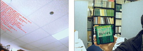
Figure 40-1 Using Computer Vision to Mediate Reality
40.3.1 Using Sequences of Fragment Programs for Computer Vision
In this section, we demonstrate how a sequence of fragment programs can work together to perform more-complex computer vision operations.
Correcting Radial Distortion
Many camera lenses cause some sort of radial distortion (also known as barrel distortion) of the image, most commonly in wide-field-of-view or low-cost lenses. There are several ways of correcting for radial distortion on the graphics hardware; we present an example of how a fragment program can be used to do so.
We begin by assuming that the displacement of a pixel due to radial distortion is x, y and is commonly modeled by:
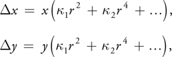
where x, y are the image coordinates, r is the distance of the pixel from the principal point of the camera, and the coefficients k 1,2,3... are camera parameters determined by some known calibration method. Given a particular camera, the required calibration parameters can be found using the tools provided at Bouguet 2004.
The fragment program shown in Listing 40-1 applies this correction by using the current texture coordinates to calculate an offset. The program then adds this offset to the current pixel's coordinates and uses the result to look up the texture value at the corrected coordinate. This texture value is then output, and the image's radial distortion is thereby corrected.
Example 40-1. Radial Undistortion
float4 CorrectBarrelDistortion(float2 fptexCoord
                               : TEXCOORD0, float4 wpos
                               : WPOS, uniform samplerRECT FPE1)
    : COLOR
{
  // known constants for the particular lens and sensor
  float f = 368.28488;
  // focal length
  float ox = 147.54834; // principal point, x axis
  float oy = 126.01673; // principal point, y axis
  float k1 = 0.4142;
  // constant for radial distortion correction
  float k2 = 0.40348;
  float2 xy = (fptexCoord - float2(ox, oy)) / float2(f, f);
  r = sqrt(dot(xy, xy));
  float r2 = r * r;
  float r4 = r2 * r2;
  float coeff = (k1 * r2 + k2 * r4);
  // add the calculated offsets to the current texture coordinates
  xy = ((xy + xy * coeff.xx) * f.xx) + float2(ox, oy);
  // look up the texture at the corrected coordinates
  // and output the color
  return texRECT(FPE1, xy);
}
A Canny Edge Detector
Edge detection is a key algorithm used in many vision applications. Here we present an implementation of the commonly used "Canny" edge-detection algorithm that runs entirely on the GPU. See Figure 40-2 for an example. We implement the Canny edge detector as a series of fragment programs, each performing a step of the algorithm:
- Step 1. Filter the image using a separable Gaussian edge filter (Jargstorff 2004). The filter footprint is typically around 15x15 elements wide, and separable. A separable filter is one whose 2D mask can be calculated by applying two 1D filters in the x and y directions. The separability saves us a large number of texture lookups, at the cost of an additional pass.
- Step 2. Determine the magnitude, l, of the derivatives at each pixel computed in
step 1, and quantize the direction d. The values of d and l are given by:
where d is the direction of the gradient vector, quantized to one of the eight possible directions one may traverse a 3x3 region of pixels. The length l is the magnitude of the vector.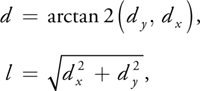
- Step 3. Perform a nonmaximal suppression, as shown in Listing 40-2. The nonmaximal suppression uses the direction of the local gradient to determine which pixels are in the forward and backward direction of the gradient. This direction is used to calculate the x and y offset of the texture coordinates to look up the forward and backward neighbors. An edge is considered found only if the gradient is at a maximum as compared to its neighbors, ensuring a thin line along the detected edge.
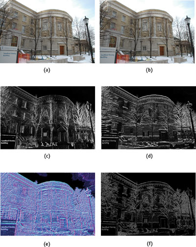
Figure 40-2 Canny Edge Detection
Example 40-2. A Canny Edge Detector Using Nonmaximal Suppression
This program looks up the direction of the gradient at the current pixel and then retrieves the pixels in the forward and backward directions along the gradient. The program returns 1 if the current pixel value is greater than the two values along the gradient; otherwise, it suppresses (or zeroes) the output. A thresholding value allows the sensitivity of the edge detector to be varied in real time to suit the vision apparatus and environment.
float4 CannySearch(uniform float4 thresh, float2 fptexCoord
                   : TEXCOORD0, uniform samplerRECT FPE1)
    : COLOR
{
  // magdir holds { dx, dy, mag, direct }
  float4 magdir = texRECT(FPE1, fptexCoord);
  float alpha = 0.5 / sin(3.14159 / 8); // eight directions on grid
  float2 offset = round(alpha.xx * magdir.xy / magdir.zz);
  float4 fwdneighbour, backneighbour;
  fwdneighbour = texRECT(FPE1, fptexCoord + offset);
  backneighbour = texRECT(FPE1, fptexCoord + offset);
  float4 colorO;
  if (fwdneighbour.z > magdir.z || backneighbour.z > magdir.z)
    colorO = float4(0.0, 0.0, 0.0, 0.0); // not an edgel
  else
    colorO = float4(1.0, 1.0, 1.0, 1.0); // is an edgel
  if (magdir.z < thresh.x)
    colorO = float4(0.0, 0.0, 0.0, 0.0); // thresholding
  return colorO;
}
40.3.2 Summation Operations
Many common vision operations involve the summation of an image buffer. Some methods that require the summation are moment calculations and the solutions to linear systems of equations.
Buck and Purcell (2004) discuss a general method of efficiently summing buffers by using local neighborhoods. On systems that do not support render-to-texture, however, the number of passes required by this technique can be limiting, due to the number of graphics context switches involved. We have found performing the computation in two passes to be more efficient on such systems. In our approach, we create a fragment program that sums each row of pixels, resulting in a single column holding the sums of each row. Then, in a second pass, we draw a single pixel and execute a program that sums down the column. The result is a single pixel that has as its "color" the sum of the entire buffer. The Cg code for computing the sum in this way is given in this chapter's appendix on the book's CD.
We use the summation operation within the context of two different, but commonly used, algorithms that require summation over a buffer: a hand-tracking algorithm and an algorithm for creating panoramas from images by determining how to stitch them together.
Tracking Hands
Tracking a user's hands or face is a useful vision tool for creating interactive systems, and it can be achieved on the GPU by using a combination of image filtering and moment calculations. A common way to track a user's hand is to use color segmentation to find areas that are skin-colored, and then continually track the location of those areas through the image. Additionally, it is useful to track the average color of the skin tone, because it changes from frame to frame, typically due to changes in lighting.
It is common to carry out the segmentation in an HSV color space, because skin tone of all hues tends to cluster in HSV color space. The HSV color space describes colors in terms of their hue (the type of color, such as red, green, or blue); saturation (the vibrancy of that color); and value (the brightness of the color). Cameras typically produce an RGB image, so a fragment program can be used to perform a fast color space conversion as a filtering operation.
Assuming that we have some sort of initial guess for the HSV color of the skin, we can also use a fragment program to threshold pixels. Given a particular pixel's HSV value, we can determine its difference from the mean HSV skin color and either output to 0 if the difference is too great or output the HSV value otherwise. For instance, the comparison might be easily done as:
if (distance(hsv, meanhsv) < thresh)
{
  colorO = hsv;
}
else
  colorO = float4(0.0, 0.0, 0.0, 0.0);
Finally, we determine the centroid of the skin-colored region and update the mean skin value based on what is currently being seen. For both of these steps, we need to calculate sums over the image.
To compute centroids, we can first compute the first three moments of the image:
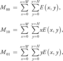
where W and H are the sizes of the image in each axis, and E (x, y) is the pixel value at location (x, y). The x coordinate of the centroid is then computed as M 10/M 00, and M 01/M 00 is the centroid's y coordinate.
These summations can be done by first running a fragment program that fills a buffer with:

and then using a GPU summation method to sum the entire buffer. The result will be a single pixel whose value can then be read back to the CPU to update the location of the centroid.
In our case—tracking the centroid of a thresholded skin-tone blob—we might simply let the fragment program output 1.0 in skin-colored areas and 0 elsewhere. Listing 40-3 shows a Cg program that produces four output components that, after summation, will provide the sums needed to calculate the zeroth and first-order moments. Figure 40-3 depicts this process.
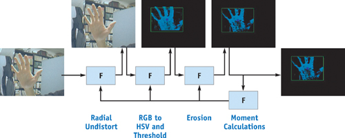
Figure 40-3 Tracking a User's Hand
Should we require more statistics like the preceding, we could either reduce the precision and output eight 16-bit floating-point results to a 128-bit floating-point texture or use the multiple render targets (MRTs) OpenGL extension.
Example 40-3. Creating Output Statistics for Moment Calculations
float4 ComputeMoments(float2 texCoord
                      : TEXCOORD0, uniform samplerRECT FPE1
                      : TEXUNIT0)
    : COLOR
{
  float4 samp = texRECT(FPE1, fptexCoord);
  float4 colorO = float4(0, 0, 0, 0);
  if (samp.x != 0.0)
    colorO = float4(1.0, fptexCoord.x, fptexCoord.y, samp.y);
}
40.3.3 Systems of Equations for Creating Image Panoramas
We also encounter this compute-and-sum type of calculation when we form systems of equations of the familiar form Ax = b.
VideoOrbits
VideoOrbits is an image-registration algorithm that calculates a coordinate transformation between pairs of images taken with a camera that is free to pan, tilt, rotate about its optical axis, and zoom. The technique solves the problem for two cases: (1) images taken from the same location of an arbitrary 3D scene or (2) images taken from arbitrary locations of a flat scene. Figure 40-4 shows an image panorama composed from several frames of video. Equivalently, Mann and Fung (2002) show how the same algorithm can be used to replace planes in the scene with computer-generated content, such as in Figure 40-1.
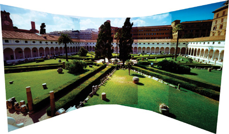
Figure 40-4 A VideoOrbits Panorama
VideoOrbits solves for a projection of an image in order to register it with another image. Consider a pair of images of the same scene, with the camera having moved between images. A given point in the scene appearing at coordinates [x, y] in the first image now appears at coordinates [x', y'] in the second image. Under the constraints mentioned earlier, all the points in the image can be considered to move according to eight parameters, given by the following equation:
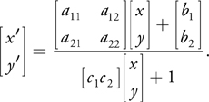
The eight scalar parameters describing the projection are denoted by:

and are calculated by VideoOrbits. Once the parameters p have been determined for each image, the images can then be transformed into the same coordinate system to create the image panoramas of Figure 40-4. (For a more in-depth treatment of projective flow and the VideoOrbits algorithm, see Mann 1998.)
VideoOrbits calculates the parameters p by solving a linear system of equations. The bulk of the computation is in the initialization of this system of equations, which is of the form Ax = b. Here, A is an 8x8 matrix whose values we must initialize, x is an 8x1 column vector that corresponds to p, and b is an 8x1 column vector we must also initialize.
Solving this system is computationally expensive because each element of A and b is actually a summation of a series of multiplications and additions at each point in the image. Initializing each of the 64 entries of the matrix A involves many multiplications and additions over all the pixels. A is of the form:
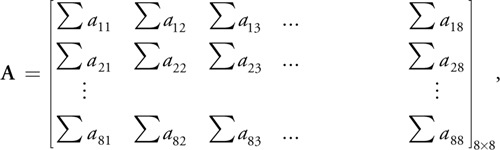
where each of the elements is a summation. (Note that the elements a 11, a 12, a 21, a 22 are not those of Equation 1.) The arguments of these summations involve many arithmetic operations. For instance, element a 21 is:

This operation must be carried out at every pixel and then summed to obtain each entry in matrix A.
This compute-and-sum operation is similar to moment calculations discussed previously. Not surprisingly, we can calculate this on the GPU in a similar fashion, filling a buffer with the argument of the summation and then summing the buffer. Typically, to calculate all the matrix entries, multiple passes will be required.
As each summation is completed, the results are copied to a texture that stores the results. After all the entries for the matrix A and vector b are computed, the values are read back to the CPU. This keeps the operations on the GPU, deferring the readback until all matrix entries have been calculated. This allows the GPU to operate with greater independence from the CPU. The system can then be solved on the CPU, with the majority of the per-pixel calculations already solved by the GPU.
40.3.4 Feature Vector Computations
Calculating feature vectors at detected feature points is a common operation in computer vision. A feature in an image is a local area around a point with some higher-than-average amount of "uniqueness." This makes the point easier to recognize in subsequent frames of video. The uniqueness of the point is characterized by computing a feature vector for each feature point. Feature vectors can be used to recognize the same point in different images and can be extended to more generalized object recognition techniques. Figure 40-5 shows the motion of the features between frames as the camera moves.
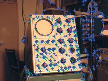
Figure 40-5 Detecting Distinctive Points as the Camera Pans
Computing feature vectors on the GPU requires handling the image data in a different manner than the operations we have thus far presented. Because only a few points in the image are feature points, this calculation does not need to be done at every point in the image. Additionally, for a single feature point, a large feature vector (100 elements or more) is typically calculated. Thus, each single point produces a larger number of results, rather than the one-to-one or many-to-one mappings we have discussed so far.
These types of computations can still be carried out on the GPU. We take as an example a feature vector that is composed of the filtered gradient magnitudes in a local region around a located feature point.
Feature detection can be achieved using methods similar to the Canny edge detector that instead search for corners rather than lines. If the feature points are being detected using sequences of filtering, as is common, we can perform the filtering on the GPU and read back to the CPU a buffer that flags which pixels are feature points. The CPU can then quickly scan the buffer to locate each of the feature points, creating a list of image locations at which we will calculate feature vectors on the GPU.
There are many approaches to generating feature vectors in order to track feature points. We show one approach as an example. For each detected feature point, we examine a 16x16 neighborhood of gradient magnitudes and directions (as computed in the Canny edge example). This neighborhood is divided up into 4x4-pixel regions, giving 16 different regions of 16 pixels. In each region, we create an 8-element histogram of gradient magnitudes. Each pixel's gradient magnitude is added to the bin of the histogram corresponding to its quantized gradient direction. For each region, the result is then an 8-element histogram. The feature vector is the concatenation of all 16 of these 8-element histograms, giving a feature vector length of 16 x 8 = 128 elements. Features in different images can be matched to each other by computing the Euclidean distance between pairs of feature vectors, with the minimum distance providing a best match.
To produce the 128-element feature vector result, we draw rows of vertices, with one row for each feature, such that each drawn point in the row corresponds to an element of the feature vector for that feature. Associating texture values pointwise allows for the most flexibility in mapping texture coordinates for use in computing the feature vector. Figure 40-6 shows how the vertices are laid out, and the binding of the image texture coordinates. Each point has different texture coordinates mapped to it to allow a single fragment program to access the appropriate gradients of the local region used to calculate the histogram.
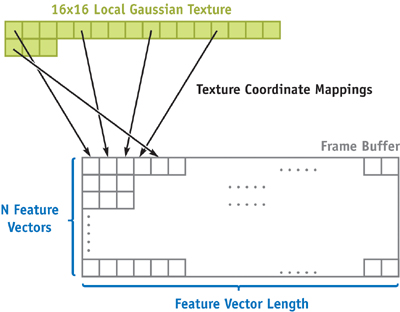
Figure 40-6 OpenGL Vertex Layout and Texture Bindings for Feature Vertices
By associating the correct texture coordinates for each point vertex, the single fragment program shown in Listing 40-4 calculates the feature vectors. To produce 8 elements per region, we have packed the results into 16-bit half-precision floating-point values; alternatively, we could use MRTs to output multiple 32-bit values. After completion, we read back the frame buffer, containing one feature vector per row, to the CPU.
Example 40-4. Fragment Program for Calculating Feature Vectors
float4 FeatureVector(float2 fptexCoord
                     : TEXCOORD0, float2 tapsCoord
                     : TEXCOORD1, float4 colorZero
                     : COLOR0, float4 wpos
                     : WPOS, uniform samplerRECT FPE1, uniform samplerRECT FPE2)
    : COLOR
{
  const float4x4 lclGauss = {0.3536, 0.3536, 0.3536, 0.3536, 0.3536, 0.7071,
                             0.7071, 0.3536, 0.3536, 0.7071, 0.7071, 0.3536,
                             0.3536, 0.3536, 0.3536, 0.3536};
  const float eps = 0.001;
  float4 input;
  int xoffset = 1, yoffset = 1;
  float4 bins_0 = float4(0.0, 0.0, 0.0, 0.0);
  float4 bins_1 = float4(0.0, 0.0, 0.0, 0.0);
  for (xoffset = 0; xoffset < 4; xoffset++)
  {
    for (yoffset = 0; yoffset < 4; yoffset++)
    {
      input = texRECT(FPE1, fptexCoord + float2(xoffset, yoffset));
      float dir = input.y;
      input *= lclGauss[xoffset, yoffset].xxxx *
               texRECT(FPE2, tapsCoord + float2(xoffset, yoffset)).xxxx;
      if (dir < = (1.0 + eps) / 8.0)
        bins_0.x += input.z;
      /* . . . for each bin . . . */
      else if (dir < = (7.0 + eps) / 8.0)
        bins_1.z += input.z;
      else
        bins_1.w += input.z;
    }
  }
  return float4(pack_2half(bins_0.xy), pack_2half(bins_0.zw),
                pack_2half(bins_1.xy), pack_2half(bins_1.zw))
}
40.4 Parallel Computer Vision Processing
When multiple computer vision algorithms are needed for an application, parallel GPU processing can be achieved by placing multiple graphics cards in the PCI bus slots of a motherboard. Figure 40-7 shows a machine built to explore the benefits of parallel computations by using multiple graphics cards. Running each computer vision program on a different GPU allows the cards to process in parallel; conventional shared memory can be used to allow the programs to interact.
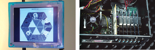
Figure 40-7 Multiple GPUs Used for a Computer Vision Application
Although creating multi-GPU systems using PCI cards will soon no longer be possible due to the obsolescence of the PCI bus, the advent of PCI Express has made new multi-GPU approaches possible. One such approach is NVIDIA's SLI, which makes the presence of multiple GPUs transparent to the developer by automatically distributing work between them.
40.5 Conclusion
This chapter has presented techniques for mapping computer vision algorithms onto modern GPUs. We hope that this chapter has provided an understanding of how to write computer vision algorithms for fast processing on the GPU. Although other special-purpose hardware systems could be used to provide hardware acceleration of computer vision algorithms, the low cost and widespread availability of GPUs will make hardware-accelerated computer vision algorithms more accessible.
40.6 References
The methods presented here are implemented in the OpenVIDIA project. OpenVIDIA is an open-source project that includes library functions and sample programs that run computer vision applications on the GPU. For more information, visit OpenVidia's Web site: http://openvidia.sourceforge.net.
Bouguet, J.-Y. 2004. Camera Calibration Toolbox for Matlab. Available online at http://www.vision.caltech.edu/bouguetj/calib_doc/index.html
Bradski, G. 1998. "Computer Vision Face Tracking for Use in a Perceptual User Interface." Intel Technology Journal.
Buck, I., and T. Purcell. 2004. "A Toolkit for Computation on GPUs." In GPU Gems, edited by Randima Fernando, pp. 621–636. Addison-Wesley.
Canny, J. F. 1986. "A Computational Approach to Edge Detection." IEEE PAMI 8(6), pp. 679–698.
Fung, J., and S. Mann. 2004a. "Computer Vision Signal Processing on Graphics Processing Units." In Proceedings of the IEEE International Conference on Acoustics, Speech, and Signal Processing (ICASSP 2004), Montreal, Quebec, Canada, pp. 83–89.
Fung, J., and S. Mann. 2004b. "Using Multiple Graphics Cards as a General Purpose Parallel Computer: Applications to Computer Vision." In Proceedings of the 17th International Conference on Pattern Recognition (ICPR2004), Cambridge, United Kingdom, pp. 805–808.
Fung, J., F. Tang, and S. Mann. 2002. "Mediated Reality Using Computer Graphics Hardware for Computer Vision." In Proceedings of the International Symposium on Wearable Computing 2002 (ISWC2002), Seattle, Washington, pp. 83–89.
Horn, B., and B. Schunk. 1981. "Determining Optical Flow." Artificial Intelligence 17, pp. 185–203.
Jargstorff, F. 2004. "A Framework for Image Processing." In GPU Gems, edited by Randima Fernando, pp. 445–467. Addison-Wesley.
Lowe, D. 2004. "Distinctive Image Features from Scale-Invariant Keypoints." International Journal of Computer Vision 60(2), pp. 91–110.
Mann, S. 1998. "Humanistic Intelligence/Humanistic Computing: 'Wearcomp' as a New Framework for Intelligent Signal Processing." Proceedings of the IEEE 86(11), pp. 2123–2151. Available online at http://wearcam.org/procieee.htm
Mann, S., and J. Fung. 2002. "Eye Tap Devices for Augmented, Deliberately Diminished or Otherwise Altered Visual Perception of Rigid Planar Patches of Real World Scenes." Presence 11(2), pp. 158–175.
Tsai, R. 1986. "An Efficient and Accurate Camera Calibration Technique for 3D Machine Vision." In Proceedings of IEEE Conference on Computer Vision and Pattern Recognition, Miami Beach, Florida, pp. 364–374.
Copyright
Many of the designations used by manufacturers and sellers to distinguish their products are claimed as trademarks. Where those designations appear in this book, and Addison-Wesley was aware of a trademark claim, the designations have been printed with initial capital letters or in all capitals.
The authors and publisher have taken care in the preparation of this book, but make no expressed or implied warranty of any kind and assume no responsibility for errors or omissions. No liability is assumed for incidental or consequential damages in connection with or arising out of the use of the information or programs contained herein.
NVIDIA makes no warranty or representation that the techniques described herein are free from any Intellectual Property claims. The reader assumes all risk of any such claims based on his or her use of these techniques.
The publisher offers excellent discounts on this book when ordered in quantity for bulk purchases or special sales, which may include electronic versions and/or custom covers and content particular to your business, training goals, marketing focus, and branding interests. For more information, please contact:
U.S. Corporate and Government Sales
(800) 382-3419
corpsales@pearsontechgroup.com
For sales outside of the U.S., please contact:
International Sales
international@pearsoned.com
Visit Addison-Wesley on the Web: www.awprofessional.com
Library of Congress Cataloging-in-Publication Data
GPU gems 2 : programming techniques for high-performance graphics and general-purpose
computation / edited by Matt Pharr ; Randima Fernando, series editor.
p. cm.
Includes bibliographical references and index.
ISBN 0-321-33559-7 (hardcover : alk. paper)
1. Computer graphics. 2. Real-time programming. I. Pharr, Matt. II. Fernando, Randima.
T385.G688 2005
006.66—dc22
2004030181
GeForce™ and NVIDIA Quadro® are trademarks or registered trademarks of NVIDIA Corporation.
Nalu, Timbury, and Clear Sailing images © 2004 NVIDIA Corporation.
mental images and mental ray are trademarks or registered trademarks of mental images, GmbH.
Copyright © 2005 by NVIDIA Corporation.
All rights reserved. No part of this publication may be reproduced, stored in a retrieval system, or transmitted, in any form, or by any means, electronic, mechanical, photocopying, recording, or otherwise, without the prior consent of the publisher. Printed in the United States of America. Published simultaneously in Canada.
For information on obtaining permission for use of material from this work, please submit a written request to:
Pearson Education, Inc.
Rights and Contracts Department
One Lake Street
Upper Saddle River, NJ 07458
Text printed in the United States on recycled paper at Quebecor World Taunton in Taunton, Massachusetts.
Second printing, April 2005
Dedication
To everyone striving to make today's best computer graphics look primitive tomorrow
- Copyright
- Inside Back Cover
- Inside Front Cover
- Part I: Geometric Complexity
-
- Chapter 1. Toward Photorealism in Virtual Botany
- Chapter 2. Terrain Rendering Using GPU-Based Geometry Clipmaps
- Chapter 3. Inside Geometry Instancing
- Chapter 4. Segment Buffering
- Chapter 5. Optimizing Resource Management with Multistreaming
- Chapter 6. Hardware Occlusion Queries Made Useful
- Chapter 7. Adaptive Tessellation of Subdivision Surfaces with Displacement Mapping
- Chapter 8. Per-Pixel Displacement Mapping with Distance Functions
- Part II: Shading, Lighting, and Shadows
-
- Chapter 9. Deferred Shading in S.T.A.L.K.E.R.
- Chapter 10. Real-Time Computation of Dynamic Irradiance Environment Maps
- Chapter 11. Approximate Bidirectional Texture Functions
- Chapter 12. Tile-Based Texture Mapping
- Chapter 13. Implementing the mental images Phenomena Renderer on the GPU
- Chapter 14. Dynamic Ambient Occlusion and Indirect Lighting
- Chapter 15. Blueprint Rendering and "Sketchy Drawings"
- Chapter 16. Accurate Atmospheric Scattering
- Chapter 17. Efficient Soft-Edged Shadows Using Pixel Shader Branching
- Chapter 18. Using Vertex Texture Displacement for Realistic Water Rendering
- Chapter 19. Generic Refraction Simulation
- Part III: High-Quality Rendering
-
- Chapter 20. Fast Third-Order Texture Filtering
- Chapter 21. High-Quality Antialiased Rasterization
- Chapter 22. Fast Prefiltered Lines
- Chapter 23. Hair Animation and Rendering in the Nalu Demo
- Chapter 24. Using Lookup Tables to Accelerate Color Transformations
- Chapter 25. GPU Image Processing in Apple's Motion
- Chapter 26. Implementing Improved Perlin Noise
- Chapter 27. Advanced High-Quality Filtering
- Chapter 28. Mipmap-Level Measurement
- Part IV: General-Purpose Computation on GPUS: A Primer
-
- Chapter 29. Streaming Architectures and Technology Trends
- Chapter 30. The GeForce 6 Series GPU Architecture
- Chapter 31. Mapping Computational Concepts to GPUs
- Chapter 32. Taking the Plunge into GPU Computing
- Chapter 33. Implementing Efficient Parallel Data Structures on GPUs
- Chapter 34. GPU Flow-Control Idioms
- Chapter 35. GPU Program Optimization
- Chapter 36. Stream Reduction Operations for GPGPU Applications
- Part V: Image-Oriented Computing
-
- Chapter 37. Octree Textures on the GPU
- Chapter 38. High-Quality Global Illumination Rendering Using Rasterization
- Chapter 39. Global Illumination Using Progressive Refinement Radiosity
- Chapter 40. Computer Vision on the GPU
- Chapter 41. Deferred Filtering: Rendering from Difficult Data Formats
- Chapter 42. Conservative Rasterization
- Part VI: Simulation and Numerical Algorithms
-
- Chapter 43. GPU Computing for Protein Structure Prediction
- Chapter 44. A GPU Framework for Solving Systems of Linear Equations
- Chapter 45. Options Pricing on the GPU
- Chapter 46. Improved GPU Sorting
- Chapter 47. Flow Simulation with Complex Boundaries
- Chapter 48. Medical Image Reconstruction with the FFT