
GPU Gems 2
GPU Gems 2 is now available, right here, online. You can purchase a beautifully printed version of this book, and others in the series, at a 30% discount courtesy of InformIT and Addison-Wesley.
The CD content, including demos and content, is available on the web and for download.
Chapter 10. Real-Time Computation of Dynamic Irradiance Environment Maps
Gary King
NVIDIA Corporation
Environment maps are a popular image-based rendering technique, used to represent spatially invariant [1] spherical functions. This chapter describes a fully GPU-accelerated method for generating one particularly graphically interesting type of environment map, irradiance environment maps, using DirectX Pixel Shader 3.0 and floating-point texturing. This technique enables applications to quickly approximate complex global lighting effects in dynamic environments (such as radiosity from dynamic lights and dynamic objects). For brevity, this chapter assumes that the reader has working knowledge of environment maps, particularly cube maps (Voorhies and Foran 1994) and dual-paraboloid maps (Heidrich and Seidel 1998).
10.1 Irradiance Environment Maps
Imagine a scene with k directional lights, with directions d 1..dk and intensities i 1..ik, illuminating a diffuse surface with normal n and color c. Given the standard OpenGL and DirectX lighting equations, the resulting pixel intensity B is computed as:
Equation 10-1 Diffuse Reflection
In this context, an environment map with k texels can be thought of as a simple method of storing the intensities of k directional lights, with the light direction implied from the texel location. This provides an efficient mechanism for storing arbitrarily complex lighting environments; however, the cost of computing B increases proportionally to the number of texels in the environment map. What we would like is a mechanism for precomputing the diffuse reflection, so that the per-pixel rendering cost is independent of the number of lights/texels.
Looking at Equation 10-1, we notice a few things: First, all surfaces with normal direction n will return the same value for the sum. Second, the sum is dependent on just the lights in the scene and the surface normal. What this means is that we can compute the sum for any normal n in an offline process executed once per environment map, and store the result in a second environment map, indexed by the surface normal. This second environment map is known as the diffuse irradiance environment map (or just the diffuse environment map), and it allows us to illuminate objects with arbitrarily complex lighting environments with a single texture lookup. (This includes natural lighting environments generated from photographs, created by Miller and Hoffman [1984], popularized by Paul Debevec [1998], and demonstrated in Figure 10-1.) Some simple pseudocode for generating diffuse environment maps [2] is shown in Listing 10-1. Figure 10-2b shows an example of a diffuse environment map.
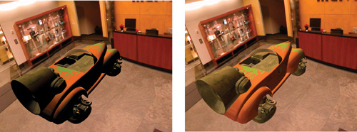
Figure 10-1 An Image Generated Using Irradiance Environment Maps
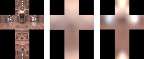
Figure 10-2 Comparing Irradiance Environment Maps
Example 10-1. Diffuse Convolution Pseudocode
diffuseConvolution(outputEnvironmentMap, inputEnvironmentMap)
{
  for_all{T0 : outputEnvironmentMap} sum = 0 N = envMap_direction(T0)
  for_all{T1 : inputEnvironmentMap} L = envMap_direction(T1) I =
      inputEnvironmentMap[T1] sum += max(0, dot(L, N)) *I T0 =
          sum return outputEnvironmentMap
}
This concept can be trivially extended to handle popular symmetric specular functions, such as the Phong reflection model. Instead of creating an irradiance environment map indexed by the surface normal, we create one indexed by the view-reflection vector R; and instead of computing max(0, dot(L, N)) for each input texel, we compute pow(max(0, dot(R, L)), s). These are known as specular irradiance environment maps.
10.2 Spherical Harmonic Convolution
Although rendering with irradiance environment maps is extremely efficient (just one lookup for a diffuse reflection or two for diffuse and specular), generating them using the algorithm in Listing 10-1 is not. For M input texels and N output texels, generating a single irradiance map is an O(MN) operation. In more concrete terms, if we want to generate a diffuse cube map with an edge length of just 32 texels, from an input cube map with an edge length of 64 texels, the cost is 32x32x6x64x64x6  151 million operations. Even with CPU speeds approaching 4 GHz, real-time generation of irradiance environment maps cannot be achieved using such a brute-force algorithm.
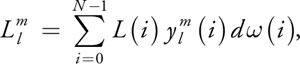
At SIGGRAPH 2001, a technique was presented that reduced the cost of computing irradiance environment maps from O(MN) to O(MK), with N>>K (Ramamoorthi and Hanrahan 2001b). The key insight was that diffuse irradiance maps vary extremely slowly with respect to the surface normal, so they could be generated and stored more efficiently by using the frequency-space representation of the environment map. To convert a spherical function (such as an environment map) into its frequency-space representation, we use the real spherical harmonic transform [3]:
Equation 10-2 Spherical Harmonic Transform
For N discrete samples (such as an environment map), Equation 10-2 becomes:
Equation 10-3 Discrete Spherical Harmonic Transform
where
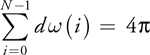
is the solid angle subtended by each sample, [4] and definitions for  (the spherical harmonic basis functions) can be found in Ramamoorthi and Hanrahan 2001b, Green 2003, or any spherical harmonics reference.
While a detailed discussion of spherical harmonics is outside the scope of this chapter, the References section lists a number of excellent articles that provide in-depth explanations (and other applications) of spherical harmonics. In order to use spherical harmonics for computing irradiance maps, all we need to know are some basic properties:
- Any band l has 2l + 1 coefficients m, defined from - l..l. Therefore, an lth-order projection has (l + 1)2 total coefficients.
- The basis functions are linear and orthonormal.
- Convolving two functions in the spatial domain is equivalent to multiplying them in the frequency domain.
The last property (known as the convolution theorem in signal-processing parlance) is an extremely powerful one, and the reason why we can use spherical harmonics to efficiently generate irradiance maps: Given two functions that we want to convolve (the Lambertian BRDF and a sampled lighting environment, for example), we can compute the convolved result by separately projecting each function into an lth-order spherical harmonic representation, and then multiplying and summing the resulting (l + 1)2 coefficients. This is more efficient than brute-force convolution because for diffuse lighting (and low-exponent specular), the  coefficients (Equation 10-3) rapidly approach 0 as l increases, so we can generate very accurate approximations to the true diffuse convolution with a very small number of terms. In fact, Ramamoorthi and Hanrahan (2001a) demonstrate that l = 2 (9 coefficients) is all that is required for diffuse lighting, and l =
  is sufficient for specular lighting (where s is the Phong exponent). This reduces the runtime complexity of the example convolution to just 9 x 64 x 64 x 6 221 thousand operations per function (442 thousand total, 1 for the lighting environment, and 1 for the reflection function), compared to the 151 million operations using the brute-force technique.
We can further improve the spherical harmonic convolution performance by noticing that the reflection function coefficients are constant for each function (Lambert, Phong, and so on). Therefore, each function's coefficients can be computed once (in a preprocess step) and be reused by all convolutions. This optimization reduces the runtime complexity of the example convolution to just 221 thousand operations.
The only remaining detail is that our diffuse environment map is now stored in a spherical harmonic representation. To convert it back into its spatial representation, [5] we generate a new environment map by using the inverse spherical harmonic transform (the tilde indicates that the reconstructed function is an approximation):
Equation 10-4 Inverse Spherical Harmonic Transform
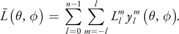
Application of this formula is trivial: for every texel in the output environment map, multiply the spherical harmonic basis function by the coefficients. This is an O(KN) process, so the total runtime complexity for generating irradiance environment maps is O(KN + KM).
10.3 Mapping to the GPU
With Pixel Shader 3.0 and floating-point textures (features supported on GeForce 6 Series GPUs), mapping spherical harmonic convolution to the GPU becomes a trivial two-pass operation [6]: one pass to transform the lighting environment into its spherical harmonic representation, and one to convolve it with the reflection function and transform it back into the spatial domain.
10.3.1 Spatial to Frequency Domain
To transform a lighting environment into its spherical harmonic representation, we need to write a shader that computes Equation 10-3. This equation has some interesting properties that can be exploited to make writing a shader a very straightforward process:
- The output is (l + 1)2 three-vector floats (one for each of red, green, and blue).
- The input is N three-vector floats, N scalar d values, and N scalar values.
- For any input texel i from any environment map L, (i)d(i) is a scalar constant.
The last point is the important one: it means that we can generate one texture per (l, m) pair as an offline process. This can then be mapped onto the GPU using (l + 1)2 rendering passes, where each pass generates a three-vector of spherical harmonic coefficients by looping over all N texels in the input environment map, and multiplying each by the corresponding texel in the appropriate lookup table. We can reduce this to a single pass by tiling the lookup tables, and rendering all of the (l + 1)2 three-vector coefficients at once, as separate pixels in an output texture. Using Pixel Shader 3.0's VPOS input register, we can trivially map the output pixel location to a tile in the lookup table, allowing each of the output pixels to project the input environment map onto the appropriate spherical harmonic basis function (scaled by d). This is shown in HLSL pseudocode in Listing 10-2 and demonstrated in Figure 10-3.
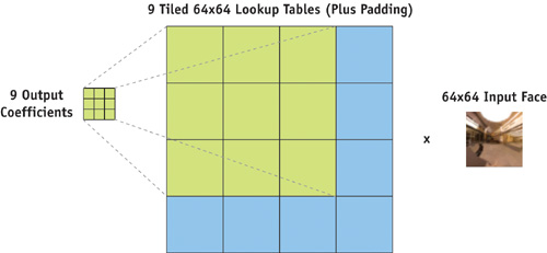
Figure 10-3 Mapping Output Coefficients to Input Lookup Table Tiles for One Face
Example 10-2. Spherical Harmonic Projection Pseudocode
float2 map_to_tile_and_offset(tile, offsetTexCoord){
    return (tile / numTiles) +
           (offsetTexCoord / (numTiles * numSamples))} float3
    SH_Projection(inputEnvironmentMap, dωYlm, currentLlm
                  : VPOS)
    : COLOR
{
  sum = 0 for_all{T0 : inputEnvironmentMap} T1 =
      map_to_tile_and_offset(currentLlm, T0) weighted_SHbasis =
          dωYlm[T1] radiance_Sample = inputEnvironmentMap[T0] sum +=
      radiance_Sample * weighted_SHbasis return sum
}
Note that for simplicity, you may want a separate lookup table for each face in the environment map. The included demo uses dual-paraboloid environment maps for input, so two weight lookup tables are generated.
10.3.2 Convolution and Back Again
As described in Section 10.2, the convolution operator in frequency space is just multiplying the coefficients generated in Section 10.3.1 with a set of precomputed coefficients for the desired reflection function (for clarity, we refer to these as the  coefficients), and then evaluating Equation 10-4 for each texel in the output environment map. This is very similar to the process we used with Equation 10-3, and we can use tiling to execute this operation in a single shader pass, too. Because is a scalar constant for any given (l, m) pair and texel location, we can precompute (l + 1)2 environment maps that store these values. If the desired output environment map is a cube map, we can instead precompute six weighting textures (one for each cube-map face), tile the (l, m) coefficients inside each face, and generate the final cube map by iteratively setting each face as the active render target, binding the appropriate weight texture, and executing the pixel shader.
The pixel shader used to perform the convolution plus inverse transformation is very similar to the one used in Section 10.3.1; however, instead of executing an N-element loop over K output values, we execute a K-element loop over M output values. Pseudocode is provided in Listing 10-3.
Example 10-3. Convolution and Evaluation Pseudocode
float3 SH_Evaluation(Llm, AlmYlm, thetaPhi : VPOS) : COLOR
{
  sum = 0
  for_all{T0 : Llm} T1 = map_to_tile_and_offset(T0, thetaPhi) weighted_BRDF =
      AlmYlm[T1] light_environment = inputEnvironmentMap[T0] sum +=
      light_environment * weighted_BRDF return sum
}
As mentioned in footnote 5, Ramamoorthi and Hanrahan (2001b) demonstrate an alternative method for performing diffuse convolution by generating a 4 x 4 matrix from the first nine terms and using this to transform the normal vector. When per-vertex lighting is sufficient, this approach may be more efficient than the one described in this chapter; however, because the convolved cube-map resolution is generally much lower than the screen resolution, the approach described here offers significant performance advantages when per-pixel lighting is desired, or in scenes with high polygon counts.
10.4 Further Work
So far, we've managed to show how to use GPUs to accelerate what is traditionally an offline process. However, because this operation executes in milliseconds on modern GPUs, by using render-to-texture functionality to generate the input environment maps, applications can practically generate diffuse and specular cube maps for dynamic environments. The accompanying demo generates irradiance maps in excess of 300 frames per second on a GeForce 6800 GT. Flat ambient lighting can be replaced with a cube-map lookup that varies as the sun moves through the sky, or as flares are tossed into a small room.
One of the deficiencies of using irradiance environment maps for scene lighting is that correct shadowing is extremely difficult, if not impossible. One technique that offline renderers use to compensate for this is computing a global shadowing term (called ambient occlusion) that is used to attenuate the illumination from the environment map (Landis 2002). For static objects, the ambient occlusion value can be precomputed and stored; however, for dynamic objects, this is not possible. In Chapter 14 of this book, "Dynamic Ambient Occlusion and Indirect Lighting," Mike Bunnell provides a method for efficiently approximating ambient occlusion values, so that this same technique can be applied to dynamic characters.
Also, spherical harmonics have a number of valuable properties not explored in this chapter. For example, component-wise linear interpolation between two sets of spherical harmonic coefficients is equivalent to linear interpolation of the spatial representations. Component-wise addition of two sets of coefficients is equivalent to addition of the spatial representations. These two properties (combined with the convolution theorem) provide a powerful set of primitives for approximating numerous complex, global lighting effects. This concept is described in detail in Nijasure 2003.
10.5 Conclusion
Rendering dynamic, complex lighting environments is an important step for interactive applications to take in the quest for visual realism. This chapter has demonstrated how one method used in offline rendering, irradiance maps, can be efficiently implemented on modern GPUs. By cleverly applying and extending the techniques presented here, real-time applications no longer need to choose between complex static lighting and simple dynamic lighting; they can have the best of both.
10.6 References
Bjorke, K. 2004. "Image-Based Lighting." In GPU Gems, edited by Randima Fernando, pp. 307–321. Addison-Wesley. This chapter describes a technique to use environment maps to represent spatially variant reflections.
Debevec, P. 1998. "Rendering Synthetic Objects into Real Scenes: Bridging Traditional and Image-Based Graphics with Global Illumination and High Dynamic Range Photography." In Computer Graphics (Proceedings of SIGGRAPH 98), pp. 189–198.
Green, R. 2003. "Spherical Harmonic Lighting: The Gritty Details." http://www.research.scea.com/gdc2003/spherical-harmonic-lighting.pdf
Heidrich, W., and H.-P. Seidel. "View-Independent Environment Maps." Eurographics Workshop on Graphics Hardware 1998, pp. 39–45.
Kautz, J., et al. 2000. "A Unified Approach to Prefiltered Environment Maps." Eurographics Rendering Workshop 2000, pp. 185–196.
Landis, H. 2002. "Production-Ready Global Illumination." Course 16 notes, SIGGRAPH 2002.
Miller, G., and C. Hoffman. 1984. "Illumination and Reflection Maps: Simulated Objects in Simulated and Real Environments." http://athens.ict.usc.edu/ReflectionMapping/illumap.pdf
Nijasure, M. 2003. "Interactive Global Illumination on the GPU." http://www.cs.ucf.edu/graphics/GPUassistedGI/GPUGIThesis.pdf
Ramamoorthi, R., and P. Hanrahan. 2001a. "A Signal-Processing Framework for Inverse Rendering." In Proceedings of SIGGRAPH 2001, pp. 117–128.
Ramamoorthi, R., and P. Hanrahan. 2001b. "An Efficient Representation for Irradiance Environment Maps." In Proceedings of SIGGRAPH 2001, pp. 497–500.
Voorhies, D., and J. Foran. 1994. "Reflection Vector Shading Hardware." In Proceedings of SIGGRAPH 94, pp. 163–166.
Copyright
Many of the designations used by manufacturers and sellers to distinguish their products are claimed as trademarks. Where those designations appear in this book, and Addison-Wesley was aware of a trademark claim, the designations have been printed with initial capital letters or in all capitals.
The authors and publisher have taken care in the preparation of this book, but make no expressed or implied warranty of any kind and assume no responsibility for errors or omissions. No liability is assumed for incidental or consequential damages in connection with or arising out of the use of the information or programs contained herein.
NVIDIA makes no warranty or representation that the techniques described herein are free from any Intellectual Property claims. The reader assumes all risk of any such claims based on his or her use of these techniques.
The publisher offers excellent discounts on this book when ordered in quantity for bulk purchases or special sales, which may include electronic versions and/or custom covers and content particular to your business, training goals, marketing focus, and branding interests. For more information, please contact:
U.S. Corporate and Government Sales
(800) 382-3419
corpsales@pearsontechgroup.com
For sales outside of the U.S., please contact:
International Sales
international@pearsoned.com
Visit Addison-Wesley on the Web: www.awprofessional.com
Library of Congress Cataloging-in-Publication Data
GPU gems 2 : programming techniques for high-performance graphics and general-purpose
computation / edited by Matt Pharr ; Randima Fernando, series editor.
p. cm.
Includes bibliographical references and index.
ISBN 0-321-33559-7 (hardcover : alk. paper)
1. Computer graphics. 2. Real-time programming. I. Pharr, Matt. II. Fernando, Randima.
T385.G688 2005
006.66—dc22
2004030181
GeForce™ and NVIDIA Quadro® are trademarks or registered trademarks of NVIDIA Corporation.
Nalu, Timbury, and Clear Sailing images © 2004 NVIDIA Corporation.
mental images and mental ray are trademarks or registered trademarks of mental images, GmbH.
Copyright © 2005 by NVIDIA Corporation.
All rights reserved. No part of this publication may be reproduced, stored in a retrieval system, or transmitted, in any form, or by any means, electronic, mechanical, photocopying, recording, or otherwise, without the prior consent of the publisher. Printed in the United States of America. Published simultaneously in Canada.
For information on obtaining permission for use of material from this work, please submit a written request to:
Pearson Education, Inc.
Rights and Contracts Department
One Lake Street
Upper Saddle River, NJ 07458
Text printed in the United States on recycled paper at Quebecor World Taunton in Taunton, Massachusetts.
Second printing, April 2005
Dedication
To everyone striving to make today's best computer graphics look primitive tomorrow
- Copyright
- Inside Back Cover
- Inside Front Cover
- Part I: Geometric Complexity
-
- Chapter 1. Toward Photorealism in Virtual Botany
- Chapter 2. Terrain Rendering Using GPU-Based Geometry Clipmaps
- Chapter 3. Inside Geometry Instancing
- Chapter 4. Segment Buffering
- Chapter 5. Optimizing Resource Management with Multistreaming
- Chapter 6. Hardware Occlusion Queries Made Useful
- Chapter 7. Adaptive Tessellation of Subdivision Surfaces with Displacement Mapping
- Chapter 8. Per-Pixel Displacement Mapping with Distance Functions
- Part II: Shading, Lighting, and Shadows
-
- Chapter 9. Deferred Shading in S.T.A.L.K.E.R.
- Chapter 10. Real-Time Computation of Dynamic Irradiance Environment Maps
- Chapter 11. Approximate Bidirectional Texture Functions
- Chapter 12. Tile-Based Texture Mapping
- Chapter 13. Implementing the mental images Phenomena Renderer on the GPU
- Chapter 14. Dynamic Ambient Occlusion and Indirect Lighting
- Chapter 15. Blueprint Rendering and "Sketchy Drawings"
- Chapter 16. Accurate Atmospheric Scattering
- Chapter 17. Efficient Soft-Edged Shadows Using Pixel Shader Branching
- Chapter 18. Using Vertex Texture Displacement for Realistic Water Rendering
- Chapter 19. Generic Refraction Simulation
- Part III: High-Quality Rendering
-
- Chapter 20. Fast Third-Order Texture Filtering
- Chapter 21. High-Quality Antialiased Rasterization
- Chapter 22. Fast Prefiltered Lines
- Chapter 23. Hair Animation and Rendering in the Nalu Demo
- Chapter 24. Using Lookup Tables to Accelerate Color Transformations
- Chapter 25. GPU Image Processing in Apple's Motion
- Chapter 26. Implementing Improved Perlin Noise
- Chapter 27. Advanced High-Quality Filtering
- Chapter 28. Mipmap-Level Measurement
- Part IV: General-Purpose Computation on GPUS: A Primer
-
- Chapter 29. Streaming Architectures and Technology Trends
- Chapter 30. The GeForce 6 Series GPU Architecture
- Chapter 31. Mapping Computational Concepts to GPUs
- Chapter 32. Taking the Plunge into GPU Computing
- Chapter 33. Implementing Efficient Parallel Data Structures on GPUs
- Chapter 34. GPU Flow-Control Idioms
- Chapter 35. GPU Program Optimization
- Chapter 36. Stream Reduction Operations for GPGPU Applications
- Part V: Image-Oriented Computing
-
- Chapter 37. Octree Textures on the GPU
- Chapter 38. High-Quality Global Illumination Rendering Using Rasterization
- Chapter 39. Global Illumination Using Progressive Refinement Radiosity
- Chapter 40. Computer Vision on the GPU
- Chapter 41. Deferred Filtering: Rendering from Difficult Data Formats
- Chapter 42. Conservative Rasterization
- Part VI: Simulation and Numerical Algorithms
-
- Chapter 43. GPU Computing for Protein Structure Prediction
- Chapter 44. A GPU Framework for Solving Systems of Linear Equations
- Chapter 45. Options Pricing on the GPU
- Chapter 46. Improved GPU Sorting
- Chapter 47. Flow Simulation with Complex Boundaries
- Chapter 48. Medical Image Reconstruction with the FFT