
GPU Gems 2
GPU Gems 2 is now available, right here, online. You can purchase a beautifully printed version of this book, and others in the series, at a 30% discount courtesy of InformIT and Addison-Wesley.
The CD content, including demos and content, is available on the web and for download.
Chapter 22. Fast Prefiltered Lines
Eric Chan
Massachusetts Institute of Technology
Frédo Durand
Massachusetts Institute of Technology
This chapter presents an antialiasing technique for lines. Aliased lines appear to have jagged edges, and these "jaggies" are especially noticeable when the lines are animated. Although line antialiasing is supported in graphics hardware, its quality is limited by many factors, including a small number of samples per pixel, a narrow filter support, and the use of a simple box filter. Furthermore, different hardware vendors use different algorithms, so antialiasing results can vary from GPU to GPU.
The prefiltering method proposed in this chapter was originally developed by McNamara, McCormack, and Jouppi (2000) and offers several advantages. First, it supports arbitrary symmetric filters at a fixed runtime cost. Second, unlike common hardware antialiasing schemes that consider only those samples that lie within a pixel, the proposed method supports larger filters. Results are hardware-independent, which ensures consistent line antialiasing across different GPUs. Finally, the algorithm is fast and easy to implement.
22.1 Why Sharp Lines Look Bad
Mathematically speaking, a line segment is defined by its two end points, but it has no thickness or area. In order to see a line on the display, however, we need to give it some thickness. So, a line in our case is defined by two end points plus a width parameter. For computer graphics, we usually specify this width in screen pixels. A thin line might be one pixel wide, and a thick line might be three pixels wide.
Before we try to antialias lines, we must understand why we see nasty aliasing artifacts in the first place. Let's say we draw a black line that is one pixel wide on a white background. From the point of view of signal processing, we can think of the line as a signal with a value of 1 corresponding to maximum intensity and 0 corresponding to minimum intensity. Because our frame buffer and display have only a finite number of pixels, we need to sample the signal. The Sampling Theorem tells us that to reconstruct the signal without aliasing, we must sample the input signal at a rate no less than twice the maximum frequency of the signal.
And that's where the problem lies. A line with perfectly sharp edges corresponds to a signal with infinitely high frequencies! We can think of an edge of a 1D line as a step function, as shown in Figure 22-1a; discrete samples are shown as vertical blue lines in Figure 22-1b. Intuitively, we can see that no matter how finely we sample this step function, we cannot represent the step discontinuity accurately enough. The three images in Figure 22-2 show what happens to the appearance of a line as we increase the pixel resolution. The results are as we expect: aliasing decreases as resolution increases, but it never goes away entirely.
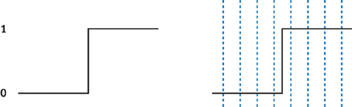
Figure 22-1 Trying to Sample a Line
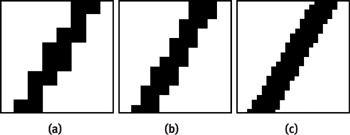
Figure 22-2 Decreasing Aliasing by Increasing Resolution
What have we learned? The only way to reconstruct a line with perfectly sharp edges is to use a frame buffer with infinite resolution—which means it would take an infinite amount of time, memory, and money. Obviously this is not a very practical solution!
22.2 Bandlimiting the Signal
A more practical solution, and the one that we describe in this chapter, is to bandlimit the signal. In other words, because we cannot represent the original signal by increasing the screen resolution, we can instead remove the irreproducible high frequencies. The visual result of this operation is that our lines will no longer appear to have sharp edges. Instead, the line's edges will appear blurry. This is what we normally think of when we hear the term "antialiased": a polygon or line with soft, smooth edges and no visible jaggies.
We can remove high frequencies from the original signal by convolving the signal with a low-pass filter. Figure 22-3 illustrates this process with a two-dimensional signal. Figure 22-3a shows the sharp edge of a line. The x and y axes represent the 2D image coordinates, and the vertical z axis represents intensity values. The left half (z = 1) corresponds to the interior of the line, and the right half (z = 0) lies outside of the line. Notice the sharp discontinuity at the boundary between z = 0 and z = 1. Figure 22-3b shows a low-pass filter, centered at a pixel; the filter is normalized to have unit volume. To evaluate the convolution of the signal in Figure 22-3a with the filter shown in Figure 22-3b at a pixel, we place the filter at that pixel and compute the volume of intersection between the filter and the signal. An example of such a volume is shown in Figure 22-3c. Repeating this process at every image pixel yields the smooth edge shown in Figure 22-3d.
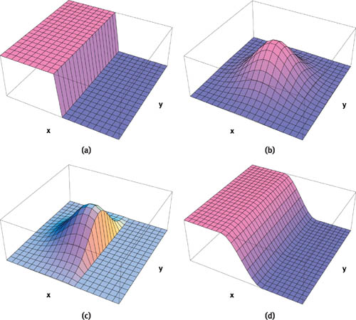
Figure 22-3 Convolution of a Sharp Line with a Low-Pass Filter
Although the idea of convolving the signal with a low-pass filter is straightforward, the calculations need to be performed at every image pixel. This makes the overall approach quite expensive! Fortunately, as we see in the next section, all of the expensive calculations can be done in a preprocess.
22.2.1 Prefiltering
McNamara et al. (2000) developed an efficient prefiltering method originally designed for the Neon graphics accelerator. We describe their method here and show how it can be implemented using a pixel shader on modern programmable GPUs.
The key observation is that if we assume that our two-dimensional low-pass filter is symmetric, then the convolution depends only on the distance from the filter to the line. This means that in a preprocess, we can compute the convolution with the filter placed at several distances from the line and store the results in a lookup table. Then at runtime, we evaluate the distance from each pixel to the line and perform a table lookup to obtain the correct intensity value. This strategy has been used in many other line antialiasing techniques, including those of Gupta and Sproull (1981) and Turkowski (1982).
This approach has several nice properties:
- We can use any symmetric filters that we like, such as box, Gaussian, or cubic filters.
- It doesn't matter if the filters are expensive to evaluate or complicated, because all convolutions are performed offline.
- The filter diameter can be larger than a pixel. In fact, according to the Sampling Theorem, it should be greater than a pixel to perform proper antialiasing. On the other hand, if we make the filter size too large, then the lines will become excessively blurry.
To summarize, this approach supports prefiltered line antialiasing with arbitrary symmetric filters at a fixed runtime cost. Now that we have seen an overview of the prefiltering method, let's dig into some of the details, starting with the preprocess.
22.3 The Preprocess
There are many questions that need to be addressed about this stage, such as how many entries in the table we need, which filter to use, and the size of the filter. We look at answers to these questions as we proceed.
Let's start by studying how to compute the table for a generic set of filter and line parameters. Figure 22-4 shows a line of width w and a filter of radius R. We distinguish between the mathematical line L, which is infinitely thin and has zero thickness, and the wide line whose edges are a distance w/2 from L. Let's ignore the line's end points for now and assume the line is infinitely long.
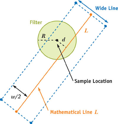
Figure 22-4 Line Configuration and Notation
When we convolve the filter with the wide line, we obtain an intensity value. Let's see what values we get by placing the filter at various distances from L. We get a maximum intensity when the filter lies directly on L, as shown in Figure 22-5a, because this is where the overlap between the filter and the wide line is maximized. Similarly, we get a minimum intensity when the filter is placed a distance of w/2 + R from the line, as shown in Figure 22-5b; this is the smallest distance for which there is no overlap between the filter and the wide line. Thus, intensity should drop off smoothly as the filter moves from a distance of 0 from L to a distance of w/2 + R.
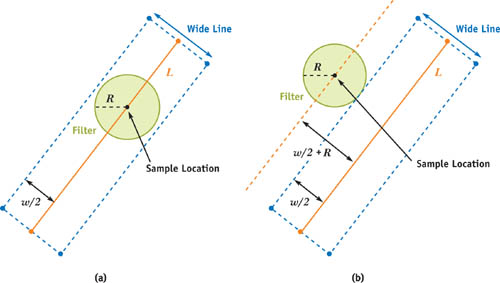
Figure 22-5 How Filter Placement Affects the Convolution
This observation turns out to be a convenient way to index the table. Instead of using the actual distance measured in pixels to index the table, we use a normalized parameter d that has a value of 1 when the filter is placed directly on L and a value of 0 when the filter is placed a distance of w/2 + R away. The reason for using this parameterization is that it allows us to handle different values for R and w in a single, consistent way.
Let's get back to some of the questions we raised earlier about prefiltering the lines. For instance, which filter should we use, and how big should it be? Signal processing theory tells us that to eliminate aliasing in the reconstructed signal, we should use the sinc filter. Unfortunately, this filter is not practical, because it has an infinite support, meaning that R would be unbounded. The good news is that we can achieve good results using simpler filters with a compact support. In practice, for thick lines (that is, with higher values of w), we prefer to use a Gaussian with a two-pixel radius and a variance of 2 = 1.0. For thinner lines, however, the results can be a bit soft and blurry, so in those cases, we use a box filter with a one-pixel radius. Blinn 1998 examines these issues in more detail. Remember, everything computed in this stage is part of a preprocess, and runtime performance is independent of our choice of filter. Therefore, feel free to precompute tables for different filters and pick one that gives results that you like.
Here's another question about our precomputation: How big do our tables need to be? Or in other words, at how many distances from L should we perform the convolution? We have found that a 32-entry table is more than enough. The natural way to feed this table to the GPU at runtime is as a one-dimensional luminance texture. A one-dimensional, 32-entry luminance texture is tiny, so if for some reason you find that 32 entries is insufficient, you can step up to a 64-entry texture and the memory consumption will still be very reasonable.
One more question before we move on to the runtime part of the algorithm: What about the line's end points? We've completely ignored them in the preceding discussion and in Figure 22-4, pretending that the line L is infinitely long. The answer is that for convenience's sake, we can ignore the end points during the preprocess and instead handle them entirely at runtime.
22.4 Runtime
The previous section covered the preprocess, which can be completed entirely on the host processor once and for all. Now let's talk about the other half of the algorithm. At runtime, we perform two types of computations. First, we compute line-specific parameters and feed them to the GPU. Second, we draw each line on the GPU conservatively as a "wide" line, and for each fragment generated by the hardware rasterizer, we use the GPU's pixel shader to perform antialiasing via table lookups. Let's dig into the details.
Each fragment produced by the rasterizer for a given line corresponds to a sample position. We need to figure out how to use this sample position to index into our precomputed lookup table so that we can obtain the correct intensity value for this fragment. Remember that our table is indexed by a parameter d that has a value of 1 when the sample lies directly on the line and a value of 0 when the sample is w/2 + R pixels away. Put another way, we need to map sample positions to the appropriate value of d. This can be done efficiently using the following line-setup algorithm.
22.4.1 Line Setup (CPU)
Let's say we want to draw the line L shown in Figure 22-6. This line is defined by its two end points (x 0, y 0) and (x 1, y 1). The actual wide line that we want to draw has width w, and its four edges surround L as shown. For a sample located at (x, y) in pixel coordinates, we can compute the parameter d efficiently by expressing d as a linear edge function of the form ax + by + c, where (a, b, c) are edge coefficients. Figure 22-6 shows four edges E 0, E 1, E 2, and E 3 surrounding L. We will compute the value of d for each edge separately and then see how to combine the results to obtain an intensity value.
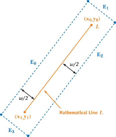
Figure 22-6 Edge Functions for a Line
First, we transform the line's end points from object space to window space (that is, pixel coordinates). This means we transform the object-space vertices by the modelview projection matrix to obtain clip-space coordinates, apply perspective division to project the coordinates to the screen, and then remap these normalized device coordinates to window space. Let (x 0, y 0) and (x 1, y 1) be the coordinates of the line's end points in window space.
Next, we compute the coefficients of the four linear edge functions. Each set of coefficients is expressed as a three-vector:
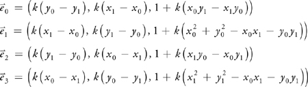
where
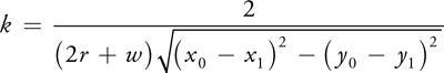
These calculations are performed once per line on the CPU.
22.4.2 Table Lookups (GPU)
The four sets of coefficients are passed to a pixel shader as uniform (that is, constant) parameters. The shader itself is responsible for performing the following calculations. If (x, y) are the pixel coordinates (in window space) of the incoming fragment, then we evaluate the four linear edge functions using simple dot products:
|
d 0 |
= |
(x, y, 1) ·
|
|
d 1 |
= |
(x, y, 1) ·
|
|
d 2 |
= |
(x, y, 1) ·
|
|
d 3 |
= |
(x, y, 1) ·
|
)
)
)
)
If any of the four results is less than zero, it means that (x, y) is more than w/2 + R pixels away from the line and therefore this fragment should be discarded.
How do we use the results of the four edge functions? We need a method that antialiases both the sides of the wide line and the end points. McNamara et al. (2000) propose the following algorithm:
intensity = lookup(min(d0, d2)) * lookup(min(d1, d3))Let's see how this method works. It finds the minimum of d 0 and d 2, the two functions corresponding to the two side edges E 0 and E 2. Similarly, it finds the minimum of d 1 and d 3, the two functions corresponding to the two end point edges E 1 and E 3 (see Figure 22-6). Two table lookups using these minimum values are performed. The lookup associated with min(d 0, d 2) returns an intensity value that varies in the direction perpendicular to L; as expected, pixels near L will have high intensity, and those near edges E 0 or E 2 will have near-zero intensity. If L was infinitely long, this would be the only lookup required.
Because we need to handle L's end points, however, the method performs a second lookup (with min(d 1, d 3)) that returns an intensity value that varies in the direction parallel to L; pixels near the end points of L will have maximum intensity, whereas those near edges E 1 and E 3 will have near-zero intensity. Multiplying the results of the two lookups yields a very close approximation to the true convolution between a filter and a finite wide line segment. The resulting line has both smooth edges and smooth end points.
Notice that only a few inexpensive operations need to be performed per pixel. This makes line antialiasing very efficient.
Cg pixel shader source code is shown in Listing 22-1. A hand-optimized assembly version requires only about ten instructions.
Example 22-1. Cg Pixel Shader Source Code for Antialiasing Lines
void main(out float4 color
          : COLOR, float4 position
          : WPOS, uniform float3 edge0, uniform float3 edge1,
            uniform float3 edge2, uniform float3 edge3, uniform sampler1D table)
{
  float3 pos = float3(position.x, position.y, 1);
  float4 d = float4(dot(edge0, pos), dot(edge1, pos), dot(edge2, pos),
                    dot(edge3, pos));
  if (any(d < 0))
    discard;
  // . . . compute color . . .
  color.w = tex1D(table, min(d.x, d.z)).x * tex1D(table, min(d.y, d.w)).x;
}
22.5 Implementation Issues
22.5.1 Drawing Fat Lines
For the pixel shader in Listing 22-1 to work, we have to make sure the hardware rasterizer generates all the fragments associated with a wide line. After all, our pixel shader won't do anything useful without any fragments! Therefore, we must perform conservative rasterization and make sure that all the fragments that lie within a distance of w/2 + R are generated. In OpenGL, this can be accomplished by calling glLineWidth with a sufficiently large value:
glLineWidth(ceil((2.0f * R + w) * sqrt(2.0f)));For example, if R = 1 and w = 2, then we should call glLineWidth with a parameter of 6. We also have to extend the line by w/2 + R in each direction to make it sufficiently long.
22.5.2 Compositing Multiple Lines
Up until now, we have only considered drawing a single line. What happens when we have multiple (possibly overlapping) lines? We need to composite these lines properly.
One way to accomplish this task is to use frame-buffer blending, such as alpha blending. In the pixel shader, we write the resulting intensity value into the alpha component of the RGBA output, as shown in Listing 22-1. In the special case where the lines are all the same color, alpha blending is a commutative operation, so the order in which we draw the lines does not matter. For the more general case of using lines with different colors, however, alpha blending is noncommutative. This means that lines must be sorted and drawn from back to front on a per-pixel basis. This cannot always be done correctly using a standard z-buffer, so instead we can use a heuristic to approximate a back-to-front sort in object space. One heuristic is to sort lines by their midpoints. Although this heuristic can occasionally cause artifacts due to incorrect sorting, the artifacts affect only a limited number of pixels and aren't particularly noticeable in practice.
22.6 Examples
Now that we've seen how to implement prefiltered lines on the GPU, let's take a look at some examples. Figure 22-7 compares hardware rendering with and without the GPU's antialiasing with the method presented in this chapter. In the first row, we draw a single black line of width 1 on an empty, white background; the second row is a close-up view of this line. In the third row, we draw a thicker black line of width 3; the fourth row provides a close-up view of the thick line. The third and fourth columns show the results of prefiltering the line using a box filter with R = 1 and a Gaussian filter with R = 2 and 2 = 1.0, respectively. The advantages in image quality of the prefiltered approach over hardware antialiasing are especially noticeable with nearly horizontal and nearly vertical lines.
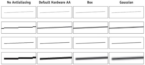
Figure 22-7 Comparing Line Antialiasing Methods for Thin and Thick Lines
An interesting application of line antialiasing is the smoothing of polygon edges. Although graphics hardware offers built-in support for polygon antialiasing, we can achieve better quality by using a simple but effective method proposed by Sander et al. (2001). The idea is first to draw the polygons in the usual way. Then we redraw discontinuity edges (such as silhouettes and material boundaries) as antialiased lines. For example, Figure 22-8a shows a single triangle drawn without antialiasing. Figure 22-8b shows its edges drawn as prefiltered antialiased lines. By drawing these lines on top of the original geometry, we obtain the result in Figure 22-8c.
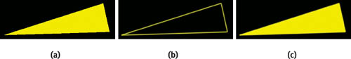
Figure 22-8 Overview of the Discontinuity Edge Overdraw Method
Comparisons showing close-ups of the triangle's nearly horizontal edge are shown in Figure 22-9. Close-ups of the triangle's nearly vertical edge are shown in Figure 22-10.
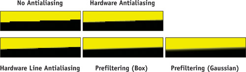
Figure 22-9 Comparing Antialiasing Methods on a Nearly Horizontal Edge
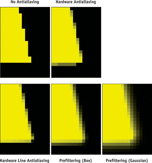
Figure 22-10 Comparing Antialiasing Methods on a Nearly Vertical Edge
There are some limitations to this polygon antialiasing approach, however. One drawback is that we must explicitly identify the discontinuity edges for a polygonal model, which can be expensive for large models. Another drawback is the back-to-front compositing issue described earlier. Standard hardware polygon antialiasing avoids these issues at the expense of image quality.
22.7 Conclusion
In this chapter we have described a simple and efficient method for antialiasing lines. The lines are prefiltered by convolving an edge with a filter placed at several distances from the edge and storing the results in a small table. This approach allows the use of arbitrary symmetric filters at a fixed runtime cost. Furthermore, the algorithm requires only small amounts of CPU and GPU arithmetic, bandwidth, and storage. These features make the algorithm practical for many real-time rendering applications, such as rendering fences, power lines, and other thin structures in games.
22.8 References
Blinn, Jim. 1998. "Return of the Jaggy." In Jim Blinn's Corner: Dirty Pixels, pp. 23–34. Morgan Kaufmann.
Gupta, Satish, and Robert F. Sproull. 1981. "Filtering Edges for Gray-Scale Devices." In Proceedings of ACM SIGGRAPH 81, pp. 1–5.
McNamara, Robert, Joel McCormack, and Norman P. Jouppi. 2000. "Prefiltered Antialiased Lines Using Half-Plane Distance Functions." In Proceedings of the ACM SIGGRAPH/Eurographics Workshop on Graphics Hardware, pp. 77–85.
Sander, Pedro V., Hugues Hoppe, John Snyder, and Steven J. Gortler. 2001. "Discontinuity Edge Overdraw." In Proceedings of the 2001 Symposium on Interactive 3D Graphics, pp. 167–174.
Turkowski, Kenneth. 1982. "Anti-Aliasing Through the Use of Coordinate Transformations." ACM Transactions on Graphics 1(3), pp. 215–234.
Copyright
Many of the designations used by manufacturers and sellers to distinguish their products are claimed as trademarks. Where those designations appear in this book, and Addison-Wesley was aware of a trademark claim, the designations have been printed with initial capital letters or in all capitals.
The authors and publisher have taken care in the preparation of this book, but make no expressed or implied warranty of any kind and assume no responsibility for errors or omissions. No liability is assumed for incidental or consequential damages in connection with or arising out of the use of the information or programs contained herein.
NVIDIA makes no warranty or representation that the techniques described herein are free from any Intellectual Property claims. The reader assumes all risk of any such claims based on his or her use of these techniques.
The publisher offers excellent discounts on this book when ordered in quantity for bulk purchases or special sales, which may include electronic versions and/or custom covers and content particular to your business, training goals, marketing focus, and branding interests. For more information, please contact:
U.S. Corporate and Government Sales
(800) 382-3419
corpsales@pearsontechgroup.com
For sales outside of the U.S., please contact:
International Sales
international@pearsoned.com
Visit Addison-Wesley on the Web: www.awprofessional.com
Library of Congress Cataloging-in-Publication Data
GPU gems 2 : programming techniques for high-performance graphics and general-purpose
computation / edited by Matt Pharr ; Randima Fernando, series editor.
p. cm.
Includes bibliographical references and index.
ISBN 0-321-33559-7 (hardcover : alk. paper)
1. Computer graphics. 2. Real-time programming. I. Pharr, Matt. II. Fernando, Randima.
T385.G688 2005
006.66—dc22
2004030181
GeForce™ and NVIDIA Quadro® are trademarks or registered trademarks of NVIDIA Corporation.
Nalu, Timbury, and Clear Sailing images © 2004 NVIDIA Corporation.
mental images and mental ray are trademarks or registered trademarks of mental images, GmbH.
Copyright © 2005 by NVIDIA Corporation.
All rights reserved. No part of this publication may be reproduced, stored in a retrieval system, or transmitted, in any form, or by any means, electronic, mechanical, photocopying, recording, or otherwise, without the prior consent of the publisher. Printed in the United States of America. Published simultaneously in Canada.
For information on obtaining permission for use of material from this work, please submit a written request to:
Pearson Education, Inc.
Rights and Contracts Department
One Lake Street
Upper Saddle River, NJ 07458
Text printed in the United States on recycled paper at Quebecor World Taunton in Taunton, Massachusetts.
Second printing, April 2005
Dedication
To everyone striving to make today's best computer graphics look primitive tomorrow
- Copyright
- Inside Back Cover
- Inside Front Cover
- Part I: Geometric Complexity
-
- Chapter 1. Toward Photorealism in Virtual Botany
- Chapter 2. Terrain Rendering Using GPU-Based Geometry Clipmaps
- Chapter 3. Inside Geometry Instancing
- Chapter 4. Segment Buffering
- Chapter 5. Optimizing Resource Management with Multistreaming
- Chapter 6. Hardware Occlusion Queries Made Useful
- Chapter 7. Adaptive Tessellation of Subdivision Surfaces with Displacement Mapping
- Chapter 8. Per-Pixel Displacement Mapping with Distance Functions
- Part II: Shading, Lighting, and Shadows
-
- Chapter 9. Deferred Shading in S.T.A.L.K.E.R.
- Chapter 10. Real-Time Computation of Dynamic Irradiance Environment Maps
- Chapter 11. Approximate Bidirectional Texture Functions
- Chapter 12. Tile-Based Texture Mapping
- Chapter 13. Implementing the mental images Phenomena Renderer on the GPU
- Chapter 14. Dynamic Ambient Occlusion and Indirect Lighting
- Chapter 15. Blueprint Rendering and "Sketchy Drawings"
- Chapter 16. Accurate Atmospheric Scattering
- Chapter 17. Efficient Soft-Edged Shadows Using Pixel Shader Branching
- Chapter 18. Using Vertex Texture Displacement for Realistic Water Rendering
- Chapter 19. Generic Refraction Simulation
- Part III: High-Quality Rendering
-
- Chapter 20. Fast Third-Order Texture Filtering
- Chapter 21. High-Quality Antialiased Rasterization
- Chapter 22. Fast Prefiltered Lines
- Chapter 23. Hair Animation and Rendering in the Nalu Demo
- Chapter 24. Using Lookup Tables to Accelerate Color Transformations
- Chapter 25. GPU Image Processing in Apple's Motion
- Chapter 26. Implementing Improved Perlin Noise
- Chapter 27. Advanced High-Quality Filtering
- Chapter 28. Mipmap-Level Measurement
- Part IV: General-Purpose Computation on GPUS: A Primer
-
- Chapter 29. Streaming Architectures and Technology Trends
- Chapter 30. The GeForce 6 Series GPU Architecture
- Chapter 31. Mapping Computational Concepts to GPUs
- Chapter 32. Taking the Plunge into GPU Computing
- Chapter 33. Implementing Efficient Parallel Data Structures on GPUs
- Chapter 34. GPU Flow-Control Idioms
- Chapter 35. GPU Program Optimization
- Chapter 36. Stream Reduction Operations for GPGPU Applications
- Part V: Image-Oriented Computing
-
- Chapter 37. Octree Textures on the GPU
- Chapter 38. High-Quality Global Illumination Rendering Using Rasterization
- Chapter 39. Global Illumination Using Progressive Refinement Radiosity
- Chapter 40. Computer Vision on the GPU
- Chapter 41. Deferred Filtering: Rendering from Difficult Data Formats
- Chapter 42. Conservative Rasterization
- Part VI: Simulation and Numerical Algorithms
-
- Chapter 43. GPU Computing for Protein Structure Prediction
- Chapter 44. A GPU Framework for Solving Systems of Linear Equations
- Chapter 45. Options Pricing on the GPU
- Chapter 46. Improved GPU Sorting
- Chapter 47. Flow Simulation with Complex Boundaries
- Chapter 48. Medical Image Reconstruction with the FFT