GPU Gems 2

GPU Gems 2 is now available, right here, online. You can purchase a beautifully printed version of this book, and others in the series, at a 30% discount courtesy of InformIT and Addison-Wesley.

The CD content, including demos and content, is available on the web and for download.

Chapter 27. Advanced High-Quality Filtering

Justin Novosad
discreet

Advanced filtering methods have been around for a long time. They were developed primarily for scientific applications such as analyzing MRIs and satellite images. Thanks to recent advances in GPU technology, these methods can be made available to PC users who simply want their computer graphics to look as nice as possible.

This chapter provides a general overview of GPU-based texture-filter implementation issues and solutions, with an emphasis on texture interpolation and antialiasing problems. We explore a series of high-quality texture-filtering methods for rendering textured surfaces. These techniques can be used to perform several common imaging tasks such as resizing, warping, and deblurring, or for simply rendering textured 3D scenes better than with the standard filters available from graphics hardware.

Readers should be familiar with the following topics: fundamental computer graphics techniques such as mipmapping, antialiasing, and texture filtering; basic frequency-domain image analysis and image processing; and calculus.

27.1 Implementing Filters on GPUs

The most practical and straightforward way to implement digital image filters on GPUs is to use pixel shaders on textured polygons. For an introduction to this approach, see Bjorke 2004. For most image-filtering applications, in which image dimensions need to be preserved, one should simply use a screen-aligned textured quad of the same dimensions as the input image.

27.1.1 Accessing Image Samples

Common digital-image-filtering methods require access to multiple arbitrary pixels from the input image. Typically, texture filters need to sample data at discrete texel locations corresponding to samples of the input image. Unfortunately, current pixel shader languages do not natively provide direct integer-addressed access to texels (except for samplerRECT in Cg). Instead, texture lookups use real coordinates in the interval 0 to 1, making lookups independent of texture resolution, which is optimal for most texture-mapping operations but not for filters. So the first step in writing a filter shader is to understand how to compute the integer sample coordinate corresponding to the current texture coordinate and how to convert sample coordinates back into conventional texture coordinates. The following equations comply with Direct3D's texture-mapping specifications:

 sampleCoord = floor(textureCoord * texSize);  textureCoord = (sampleCoord + 0.5) / texSize;

We add 0.5 to the sample coordinates to get the coordinate of the center of the corresponding texel. Although the coordinates of texel corners could be used, it is always safer to use centers to guard against round-off errors. Variable texSize is a uniform value containing the dimensions of the texture excluding border texels.

In many situations, filters need to access only those pixels in their immediate neighborhood, in which case coordinate conversions may not be necessary. The following macros can be used to compute the texture coordinates of adjacent pixels in a single arithmetic operation:

 #define TC_XMINUS_YMINUS(coord) (coord - texIncrement.xy)  #define TC_XPLUS_YPLUS(coord) (coord + texIncrement.xy)  #define TC_XCENTER_YMINUS(coord) (coord - texIncrement.zy)  #define TC_XCENTER_YPLUS(coord) (coord + texIncrement.zy)  #define TC_XMINUS_YCENTER(coord) (coord - texIncrement.xz)  #define TC_XPLUS_YCENTER(coord) (coord + texIncrement.xz)    #define TC_XMINUS_YPLUS(coord) (coord - texIncrement.xw)  #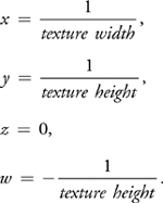define TC_XPLUS_YMINUS(coord) (coord + texIncrement.xw)

Here, texIncrement is a uniform variable whose components are initialized as follows:

One additional tip is that it is not necessary to snap texture coordinates to the center of the nearest texel as long as texture lookups do not perform any type of filtering. This means setting filtering to GL_NEAREST in OpenGL or D3DTEXF_POINT in Direct3D. This way, coordinate snapping is performed automatically during texture lookups.

27.1.2 Convolution Filters

In Bjorke 2004, as well as in Rost 2004, there are some interesting techniques for implementing convolution filters in shaders. In most situations, storing the convolution coefficients in constants or uniforms works well and is very efficient for conventional discrete convolution. However, we would like to promote the usage of textures for representing continuous convolution kernels that are required for subpixel filtering.

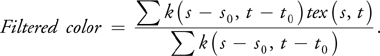
Subpixel filtering is an important tool for achieving high-quality filtered texture magnification. The idea is simple: we want to apply the convolution kernel centered precisely at the current texture coordinates, which is not necessarily at the center of a texel. In this case, the kernel must be viewed as a continuous function k(s, t). Hence, the convolution can be represented as follows:

Filtered color = k(s – s ₀, t – t ₀)tex(s, t),

where the summation is over the neighborhood of the current texel coordinate (s ₀, t ₀), and tex is the texture lookup function. In this chapter, we use (i, j) to designate screen coordinates and (s, t) to designate image and texture coordinates.

In image processing, it is often desirable to work with filters that have a steady-state response of 1, to preserve the image's mean intensity. Therefore, we want the sum of kernel coefficients to be 1, as shown in Figure 27-1.

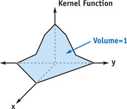
Figure 27-1 A Kernel with Unit Volume

In continuous convolution, we want to ensure that the integral of the kernel over its domain is 1. In the case of subpixel filtering, it is not that simple, because we are using a continuous kernel on a discrete image. So the kernel will have to be sampled. As a consequence, the summation of kernel samples may not be constant. The solution is to divide the resulting color by the sum of kernel samples, which gives us the following equation:

Listing 27-1 is an example of an HLSL pixel shader that performs subpixel filtering. In Listing 27-1, the convolution summation is performed in the RGB channels, while the kernel sample summation is done in the alpha channel. This little trick saves a lot of GPU instructions and helps accelerate the process. If the alpha channel needs to be processed, the kernel sample summation will have to be done separately. The variable fact is a scale factor that will convert texture coordinate offsets from the image frame of reference to kernel texture coordinates. The value of fact should be computed as image size divided by filter domain. We add 0.5 to the filter lookup coordinates because we assume that the origin of the kernel is at the center of the Filter texture.

Notice in Figure 27-2 how the subpixel Gaussian yields a nice and smooth interpolation. Unfortunately, this quality comes at a high computational cost, which is likely to make fragment processing the bottleneck in the rendering pipeline.

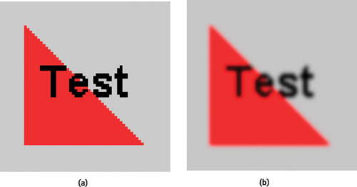
Figure 27-2 The Result of Using a Subpixel Gaussian Filter for Image Magnification

Example 27-1. Discrete Convolution with a Continuous Kernel

 int2 texSize;  half2 fact;  sampler2D Filter;  sampler2D Image;  const half pi = 3.141592654;    half4 ps_main( half4 inTex: TEXCOORD0 ) : COLOR0    {    half4 color = half4(0, 0, 0, 0);    half2 base = floor(inTex * texSize);    half2 pos;    half2 curCoord;    for (pos.x = -3; pos.x <= 3; pos.x++)    for (pos.y = -3; pos.y <= 3; pos.y++)    {      curCoord = (base + pos + 0.5) / texSize;      color += half4(tex2D(Image, curCoord).rgb, 1)*                     tex2D(Filter, (inTex - curCoord) * fact + 0.5).r;     }     return color / color.a;  }

Using 1D Textures for Rotationally Invariant Kernels

Representing in 2D a kernel that is invariant to rotation is highly redundant. All the necessary information could be encoded into a 1D texture by simply storing a cross section of the kernel. To apply this technique, replace the color summation line in Listing 27-1 with the following:

 color += half4(tex2D(Image, curCoord).rgb,1) *                 tex1D(Filter, length(inTex - curCoord) * fact).r;

This method requires us to add an expensive length() function call to the inner loop, which will likely hinder the performance of the shader, although it saves texture memory. Trading performance for texture memory is not so relevant with recent GPUs—which are typically equipped with 128 MB or more memory—unless we are dealing with very large kernels. We discuss that situation briefly in the next section.

Another, more efficient method is to take advantage of the separability of convolution kernels. A 2D convolution filter is said to be separable when it is equivalent to applying a 1D filter on the rows of the image, followed by a 1D filter on the columns of the image. The Gaussian blur and the box filter are examples of separable kernels. The downside is that the filter has to be applied in two passes, which may be slower than regular 2D convolution when the kernel is small.

Applying Very Large Kernels

Because some GPUs can execute only a relatively limited number of instructions in a shader, it may not be possible to apply large kernels in a single pass. The solution is to subdivide the kernel into tiles and to apply one tile per pass. The ranges of the two loops in Listing 27-1 must be adjusted to cover the current tile. The results of all the passes must be added together by accumulating them in the render target, which should be a floating-point renderable texture (a pbuffer in OpenGL), or an accumulation buffer. The convolution shader must no longer perform the final division by the kernel sample sum (the alpha channel), because the division can only be done once all the samples have been accumulated. The division has to be performed in a final post-processing step.

27.2 The Problem of Digital Image Resampling

In this section we look at methods for improving the visual quality of rendered textures using interpolation filters and antialiasing. We also present a method for restoring sharp edges in interpolated textures.

27.2.1 Background

A digital image is a two-dimensional array of color samples. To display a digital image on a computer screen, often the image must be resampled to match the resolution of the screen. Image resampling is expressed by the following equation:

P(i, j) = I(f(i, j)),

where P(i, j) is the color of the physical pixel at viewport coordinates (i, j); I(u, v) is the image color at coordinates (u, v); and function f maps screen coordinates to image coordinates (or texture coordinates) such that (u, v) = f(i, j). The topic we want to address is how to evaluate I(u, v) using pixel shaders to obtain high-quality visual results.

The function f(i, j) is an abstraction of the operations that go on in the software, the operating system, the graphics driver, and the graphics hardware that result in texture coordinates (u, v) being assigned to a fragment at screen coordinates (i, j). These computations are performed upstream of the fragment-processing stage, which is where I(u, v) is typically evaluated by performing a texture lookup.

OpenGL and Direct3D have several built-in features for reducing the artifacts caused by undersampling and oversampling. Undersampling occurs when the image is reduced by f, which may cause aliasing artifacts. Oversampling occurs when the image is enlarged by f, which requires sample values to be interpolated. Texture-aliasing artifacts can be eliminated through texture mipmapping, and sample interpolation can be performed using hardware bilinear filtering. Most GPUs also provide more advanced techniques, such as trilinear filtering and anisotropic filtering, which efficiently combine sample interpolation with mipmapping.

27.2.2 Antialiasing

Aliasing is a phenomenon that occurs when the Sampling Theorem, also known as Nyquist's rule, is not respected. The Sampling Theorem states that a continuous signal must be sampled at a frequency greater than twice the upper bound of the signal spectrum, or else the signal cannot be fully reconstructed from the samples (that is, information is lost). When aliasing occurs, the part of the signal spectrum that is beyond the sampling bandwidth gets reflected, which causes undesirable artifacts in the reconstructed signal (by bandwidth, we mean the frequency range allowed by Nyquist's rule). The theory behind the phenomenon of spectral aliasing is beyond the scope of this chapter; more on the topic can be found in any good signal-processing textbook.

The classic approach to antialiasing is to filter the signal to be sampled to eliminate frequency components that are beyond the sampling bandwidth. That way, the high-frequency components of the signal remain unrecoverable, but at least the low-frequency components aren't corrupted by spectral reflection. One of the best-known ways of doing this is mipmapping, which provides prefiltered undersampled representations of the texture. Mipmapping is great for interactive applications such as games, but it is not ideal, because it does not achieve optimal signal preservation, even with trilinear or anisotropic filtering.

Quasi-Optimal Antialiasing

Ideal antialiasing consists in computing sample values as the average of the sampled signal over the sampling area, which is given by the integral of the sampled signal over the sampling area divided by the sampling area. In the case of texture mapping, the sampled signal is discrete, meaning that the integral can be computed as a summation. To compute the summation, we must devise a method to determine which texels belong to the sampling area of a given pixel.

Assuming that pixels are spaced by 1 unit in both x and y directions, the screen-space corners of the sampling area of the pixel at (i, j) are (i - 0.5, j - 0.5), (i + 0.5, j - 0.5), (i + 0.5, j + 0.5), and (i - 0.5, j + 0.5). We want to compute the mapping of the sampling area in texture space. This is difficult to solve in the general case, so we propose a solution that is valid under the assumption that f(i, j) is a linear 2D vector function—hence, quasi-optimal antialiasing. Because we know that in the general case, f(i, j) is not linear, ^[1] we approximate the function locally for each pixel using the two first terms of its Taylor series expansion:

f(i, j) [s₀, t₀]^r + J₀[i–i₀, j–j₀]^r,

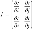
where (i ₀, j ₀) are the coordinates of the center of the current pixel; (s ₀, t ₀) is the value of f(i ₀, j ₀); J is the texture-coordinate Jacobian matrix; and J ₀ is the Jacobian matrix evaluated at the center of the current pixel.

It is a known property of linear transformations that linearity is preserved; therefore, the square sampling area is guaranteed to map to a quadrilateral in texture space. To implement texture antialiasing as a pixel shader, we will scan through each texel in the bounding box of the mapped quadrilateral and test it to determine whether it is within the quadrilateral. Another approach would be to use an edge-walking rasterization-style algorithm to select pixels. This would be more efficient for covering very large quadrilaterals, but it is too complex for GPUs that do not have advanced flow control (GPUs prior to the GeForce 6 Series).

There are several ways to test whether a pixel belongs to a quadrilateral. The one we propose here is to use the reciprocal of f to convert texture coordinates back to screen coordinates, where the test is much easier to perform. See Figure 27-3. The reciprocal function is this:

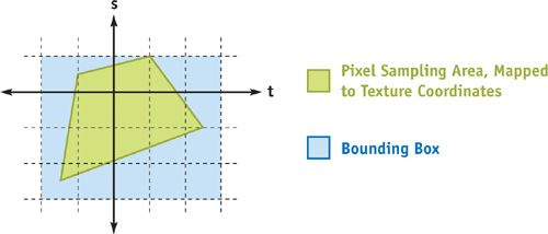
Figure 27-3 Testing Whether a Pixel Belongs to a Quadrilateral

In pixel coordinates, all we have to verify is that |i- i ₀| and |j- j ₀| are smaller than 0.5.

Listing 27-2 is a basic pixel shader that performs antialiased texture mapping that can be run on a Pixel Shader 2.0a target.

In this example, we use intrinsic function fwidth to quickly compute a conservative bounding box without having to transform the corners of the sampling area. The drawback of this approach is that it will generate bounding boxes slightly larger than necessary, resulting in more samples being thrown out by the quadrilateral test. Another particularity of this shader is that it divides the bounding box into a fixed number of

Example 27-2. A Quasi-Optimal Antialiasing Pixel Shader

 bool doTest;  int2 texSize;  sampler2D Image;  const int SAMPLES = 5;  // should be an odd number  const int START_SAMPLE = -2; // = -(SAMPLES-1)/2    // Compute the inverse of a 2-by-2 matrix  float2x2 inverse (float2x2 M)  {    return float2x2(M[1][1], -M[0][1], -M[1][0], M[0][0]) / determinant(M);  }    float4 ps_main( float2 inTex: TEXCOORD0 ) : COLOR0    {    float2 texWidth = fwidth(inTex);    float4 color = float4(0, 0, 0, 0);    float2 texStep = texWidth / SAMPLES;    float2 pos = START_SAMPLE * texStep;    float2x2 J = transpose(float2x2(ddx(inTex), ddy(inTex)));    float2x2 Jinv = inverse(J);    for (int i = 0; i < SAMPLES; i++, pos.x += texStep.x)    {      pos.y = START_SAMPLE * texStep.y;      for (int j = 0; j < SAMPLES; j++, pos.y += texStep.y)      {        float2 test = abs(mul(Jinv, pos));        if (test.x < 0.5h && test.y < 0.5h)          color += float4(tex2D(Image, inTex + pos).rgb, 1);      }    }    return color / (color.a);  }

rectangular subdivisions, which are not likely to have one-to-one correspondence with texels. Using advanced flow control, it is possible to improve the shader by making it use a variable-size texel-aligned sampling grid. See Figures 27-4 and 27-5.

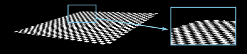
Figure 27-4 Checkerboard Texture Using Quasi-Optimal Antialiasing

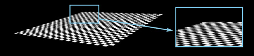
Figure 27-5 Antialiased Checkerboard Texture Without Quadrilateral Test

Figure 27-5 is the result of sampling the texture over the window given by fwidth, which is a primitive form of anisotropic filtering. The difference is subtle, but by looking at the images closely, we see that the benefit of the quasi-optimal antialiasing method is a sharper perspective texture mapping. Also note that antialiasing is applied only to the texture, not to the polygon, which explains why the outer edges of the textured quad are still jaggy. To smooth polygon edges, hardware multisampling (that is, full-scene antialiasing) should be used.

27.2.3 Image Reconstruction

When oversampling (enlarging) an image, the strategy is to reconstruct the original continuous signal and to resample it in a new, higher resolution. Bilinear texture filtering is a very quick way to do this, but it results in poor-quality, fuzzy images. In this subsection, we see how to implement some more-advanced image-reconstruction methods based on information theory.

First let's look at the Shannon-Nyquist signal reconstruction method, which can yield a theoretically perfect reconstruction of any signal that respects the Nyquist limit. The theoretical foundation of the method can be found in Jähne 2002. To apply the method in a shader, simply use the following equation to generate a subpixel convolution kernel and apply it to the texture using the shader presented in Listing 27-1.

This kernel is in fact an ideal low-pass filter, also known as the sine cardinal, or sinc for short. The simplest way to explain Shannon-Nyquist reconstruction is that it limits the spectrum of the reconstructed signal to the bandwidth of the original sampling while preserving all frequency components present in the sampled signal.

Implementation

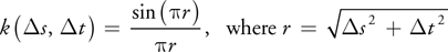
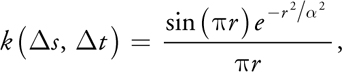
The kernel used in Shannon-Nyquist reconstruction is invariant to rotation, so we have the option of storing it as a 1D texture. However, the impulse response is infinite and dampens very slowly, as can be seen in Figure 27-6.

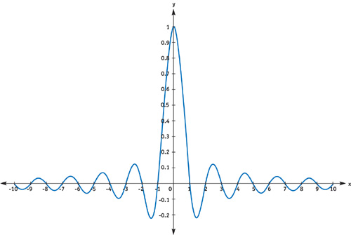
Figure 27-6 Plot of = sin()/

To achieve acceptable performance, it is important to restrict the domain of the impulse response. A common practice is to dampen the function by multiplying it with a windowing function, for example a Gaussian. The resulting filter has a compact kernel, but it is no longer an ideal low-pass filter; the frequency-response step is somewhat smoother. When multiplying with a Gaussian, the impulse response will no longer have an integral of 1; but there is no reason to bother with finding a scale factor to normalize the impulse response, because the shader takes care of all this.

Let's use the following function as our kernel:

where is a domain scale factor that must be proportional to the size of the kernel. As a rule of thumb, should be around 75 percent of the range of the kernel. Figure 27-7 shows a cross section of k with = 6, which would be appropriate for a kernel with a domain of [-8, 8].

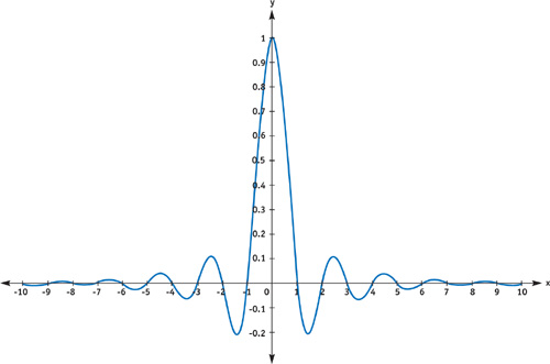
Figure 27-7 Plot of = sin()e/

Figure 27-8 shows that Shannon-Nyquist reconstruction performs very nicely on natural images but produces resonation artifacts along very sharp edges, which are more likely to occur in synthetic images. The resonation is a result of the lack of high-frequency information that is necessary to accurately define an image-intensity step in the resampled image. For processing synthetic images, it is usually preferable to simply use a Gaussian kernel. The Gaussian filter will not produce any resonating artifacts, but it will degrade fine details in the image because of its very smooth frequency cutoff, which attenuates the high-frequency components in the image. (See the results in Section 27.1.2.)

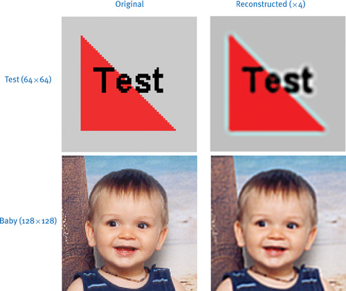
Figure 27-8 Examples of Shannon-Nyquist Image Reconstruction

27.3 Shock Filtering: A Method for Deblurring Images

The absence of high-frequency components in an image makes it harder for observers to discern objects, because the ganglion cells, which link the retina to the optic nerve, respond acutely to high-frequency image components (see the Nobel-prize-winning work of Hubel and Wiesel [1979]). Because of this, the brain's visual cortex will lack the information it requires to discern objects in a blurry image. Sharpening a blurred image (thereby recovering those high-frequency components) can greatly enhance its visual quality.

Many traditional digital-image-sharpening filters amplify the high-frequency components in an image, which may enhance visual quality. In this section, we look at a different type of sharpening filter that is more appropriate for enhancing reconstructed images: the shock filter, which transforms the smooth transitions resulting from texture interpolation into abrupt transitions. The mathematical theory behind shock filtering is clearly presented in Osher and Rudin 1990. The underlying principle is based on diffusing energy between neighboring pixels. In areas of the image where the second derivative is positive, pixel colors are diffused in the reverse gradient direction, and vice versa. To sharpen an image properly, many passes are usually required.

This method is difficult to apply to images of textured 3D scenes because blurriness may be anisotropic and uneven due to varying depth and perspective texture mapping. This is a problem because the shock-filtering algorithm has no knowledge of the distribution of blurriness in the image. Shock filtering is nonetheless of considerable interest for many types of 2D applications, where blur is often uniform. Listing 27-3 is a simple pixel shader that uses centered differences to estimate the image gradient and a five-sample method to determine convexity (the sign of the second derivative).

Example 27-3. Shock Filter Pixel Shader

 uniform float shockMagnitude;  uniform int2 destSize;  sampler2D Image;  const float4 ones = float4(1.0, 1.0, 1.0, 1.0);      float4 ps_main( float4 inTex : TEXCOORD0 ) : COLOR0  {    float3 inc = float3(1.0/destSize, 0.0); // could be a uniform      float4 curCol = tex2D(Image, inTex);    float4 upCol = tex2D(Image, inTex + inc.zy);    float4 downCol = tex2D(Image, inTex - inc.zy);    float4 rightCol = tex2D(Image, inTex + inc.xz);    float4 leftCol = tex2D(Image, inTex - inc.xz);    float4 Convexity = 4.0 * curCol - rightCol - leftCol - upCol - downCol;    float2 diffusion = float2(dot((rightCol - leftCol) * Convexity, ones),                              dot((upCol - downCol) * Convexity, ones));      diffusion *= shockMagnitude/(length(diffusion) + 0.00001);    curCol += (diffusion.x > 0 ? diffusion.x * rightCol :               -diffusion.x*leftCol) +              (diffusion.y > 0 ? diffusion.y * upCol :               -diffusion.y * downCol);    return curCol/(1 + dot(abs(diffusion), ones.xy));  }

The images in the right column in Figure 27-9 were generated with eight passes of shock filtering with the magnitude parameter set to 0.05.

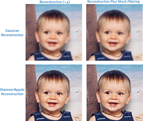
Figure 27-9 Shock Filtering

Notice that the edges of the images are generally sharper after shock filtering. Grainy textures and fine details are better preserved with Shannon-Nyquist reconstruction thanks to the sharp spectrum cutoff. However, there are shadowy artifacts around object silhouettes. The Gaussian reconstruction produces no artifacts, and a more aesthetically pleasing result, but the fine details in the image are attenuated.

27.4 Filter Implementation Tips

In many situations, shaders need to evaluate complex functions. Performance of a shader is generally closely related to the number of operations that are performed, so it is important to precompute everything that can be precomputed. Shader developers often encounter this limitation and try to use uniform variables and constants wherever possible to pass precomputed data. One particular strategy that is often overlooked is to use textures as lookup tables in order to evaluate functions quickly by performing a simple texture read instead of evaluating a complicated expression.

Here is a list of tips to consider when designing a shader that uses textures as function lookup tables:

Choose your texture format carefully, according to the desired precision and range of your function.
Scale your function properly, so that useful parts fit into the bounds of the texture. For periodic functions, use texture-coordinate wrapping. For functions with horizontal asymptotes, use texture-coordinate clamping.
Use linear texture filtering to get better precision through interpolation.
Set the resolution of your texture carefully, to make a reasonable compromise between precision and texture-memory consumption.
Not all GPUs allow linear texture filtering with floating-point textures. When filtering is not available, a higher-resolution texture may be necessary to achieve the required precision.
Whenever possible, use the different color components of the texture to evaluate several functions simultaneously.

27.5 Advanced Applications

In this section, we expose some ideas on how to use the techniques presented earlier in the chapter. These suggestions are intended for readers who wish to extend the functionality of the presented shaders to perform advanced image-processing tasks.

27.5.1 Time Warping

We have seen how subpixel convolution filtering can be used for image reconstruction, but it is also possible to generalize the method to higher-dimensional signals. By representing a sequence of images as a 3D array, the third dimension being time, it is possible to interpolate frames to yield fluid slow-motion effects. The frames of the original image sequence can be passed to the shader either as a 3D texture or as multiple 2D textures. For superior interpolation of sequences with fast-moving objects, be sure to use Shannon-Nyquist reconstruction with a very large kernel.

This technique may be considered an interesting compromise between the simple but low-quality frame-blending method and the high-quality but complex motion-estimation approach.

27.5.2 Motion Blur Removal

A slow-motion time warp by means of signal reconstruction may yield motion blur that corresponds to shutter speeds slower than the interpolated frame intervals. In such cases, one may use an adapted shock filter that diffuses only along the time dimension to attenuate motion blur.

27.5.3 Adaptive Texture Filtering

A smart and versatile shader for high-quality rendering of textured 3D scenes would combine the antialiasing and reconstruction filters presented in this chapter into one shader, which would choose between the two using a minification/magnification test. A good example of how to perform this test is given in the OpenGL specifications at http://www.opengl.org.

27.6 Conclusion

The techniques presented in this chapter are designed to produce optimal-quality renderings of 2D textures. Despite the simplicity of these techniques, their computational cost is generally too high to use them at render time in full-screen computer games and interactive applications that require high frame rates. They are more likely to be useful for applications that prioritize render quality over speed, such as medical and scientific imaging, photo and film editing, image compositing, video format conversions, professional 3D rendering, and so on. They could also be used for resolution-dependent texture preparation (preprocessing) in games.

These techniques are feasible in multimedia applications today thanks to the recent availability of highly programmable GPUs. Before, most image-processing tasks had to be performed by the CPU or by highly specialized hardware, which made advanced image-filtering methods prohibitively slow or expensive.

27.7 References

Aubert, Gilles, and Pierre Kornprobst. 2002. Mathematical Problems in Image Processing. Springer.

Bjorke, Kevin. 2004. "High-Quality Filtering." In GPU Gems, edited by Randima Fernando, pp. 391–415. Addison-Wesley.

Hubel, D. H., and T. N. Wiesel. 1979. "Brain Mechanisms of Vision." Scientific American 241(3), pp. 150–162.

Jähne, Bernd. 2002. Digital Image Processing. Springer.

Osher, S., and L. Rudin. 1990. "Feature-Oriented Image Enhancement Using Shock Filters." SIAM Journal on Numerical Analysis 27(4), pp. 919–940.

Rost, R. 2004. OpenGL Shading Language. Chapter 16. Addison-Wesley.

Copyright

Many of the designations used by manufacturers and sellers to distinguish their products are claimed as trademarks. Where those designations appear in this book, and Addison-Wesley was aware of a trademark claim, the designations have been printed with initial capital letters or in all capitals.

The authors and publisher have taken care in the preparation of this book, but make no expressed or implied warranty of any kind and assume no responsibility for errors or omissions. No liability is assumed for incidental or consequential damages in connection with or arising out of the use of the information or programs contained herein.

NVIDIA makes no warranty or representation that the techniques described herein are free from any Intellectual Property claims. The reader assumes all risk of any such claims based on his or her use of these techniques.

The publisher offers excellent discounts on this book when ordered in quantity for bulk purchases or special sales, which may include electronic versions and/or custom covers and content particular to your business, training goals, marketing focus, and branding interests. For more information, please contact:

U.S. Corporate and Government Sales
(800) 382-3419
corpsales@pearsontechgroup.com

For sales outside of the U.S., please contact:

International Sales
international@pearsoned.com

Visit Addison-Wesley on the Web: www.awprofessional.com

Library of Congress Cataloging-in-Publication Data

GPU gems 2 : programming techniques for high-performance graphics and general-purpose
computation / edited by Matt Pharr ; Randima Fernando, series editor.
p. cm.
Includes bibliographical references and index.
ISBN 0-321-33559-7 (hardcover : alk. paper)
1. Computer graphics. 2. Real-time programming. I. Pharr, Matt. II. Fernando, Randima.

T385.G688 2005
006.66—dc22
2004030181

GeForce™ and NVIDIA Quadro® are trademarks or registered trademarks of NVIDIA Corporation.

mental images and mental ray are trademarks or registered trademarks of mental images, GmbH.

All rights reserved. No part of this publication may be reproduced, stored in a retrieval system, or transmitted, in any form, or by any means, electronic, mechanical, photocopying, recording, or otherwise, without the prior consent of the publisher. Printed in the United States of America. Published simultaneously in Canada.

For information on obtaining permission for use of material from this work, please submit a written request to:

Pearson Education, Inc.
Rights and Contracts Department
One Lake Street
Upper Saddle River, NJ 07458

Text printed in the United States on recycled paper at Quebecor World Taunton in Taunton, Massachusetts.

Second printing, April 2005

Dedication

To everyone striving to make today's best computer graphics look primitive tomorrow

Part II: Shading, Lighting, and Shadows

Part III: High-Quality Rendering

Part IV: General-Purpose Computation on GPUS: A Primer

Part V: Image-Oriented Computing

Part VI: Simulation and Numerical Algorithms