GPU Gems 2

GPU Gems 2 is now available, right here, online. You can purchase a beautifully printed version of this book, and others in the series, at a 30% discount courtesy of InformIT and Addison-Wesley.

The CD content, including demos and content, is available on the web and for download.

Chapter 39. Global Illumination Using Progressive Refinement Radiosity

Greg Coombe
University of North Carolina at Chapel Hill

Mark Harris
NVIDIA Corporation

With the advent of powerful graphics hardware, people have begun to look beyond local illumination models toward more complicated global illumination models, such as those made possible by ray tracing and radiosity. Global illumination, which incorporates interobject effects such as shadows and interreflections, attains a compelling level of visual realism that is difficult to achieve with local illumination models.

In this chapter we describe a method for computing radiosity that performs all of the computation on the GPU. The radiosity energy is stored in texels, and fragment programs are used to compute the form factors and interobject visibility. We avoid the problem of writing to arbitrary locations in memory by casting progressive refinement radiosity as a "gather" operation, which has a regular memory access pattern that is amenable to running on current GPUs.

Figure 39-1 shows an image rendered in our system that demonstrates the compelling effects that can be obtained with global illumination, such as soft shadows and indirect lighting.

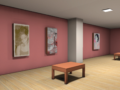
Figure 39-1 A Scene with a GPU-Accelerated Radiosity Solution

39.1 Radiosity Foundations

Radiosity is a finite-element approach to the problem of global illumination (Cohen and Wallace 1993). It breaks the scene into many small elements and calculates how much energy is transferred between the elements. The fraction of energy transferred between each pair of elements is described by an equation called the form factor. Here is a simple version of a form factor equation (Cohen and Wallace 1993), giving the form factor between two differential areas on surfaces in the scene:

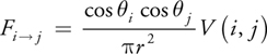
The equation is composed of two parts: a visibility term and a geometric term. The geometric term states that the fraction of energy transferred between the elements i and j is a function of the distance and relative orientation of the elements. The visibility term V(i, j) is 0 for elements that are occluded and 1 for elements that are fully visible from each other.

This formula is accurate only if i and j are infinitesimal areas (or are far enough apart to be treated as such). However, to increase the speed of the computation, we would like to use large-area elements, which break this assumption. One way to deal with large-area elements is to explicitly integrate over the area of the element. Because this is computationally expensive, we can approximate these large elements with oriented discs (Wallace et al. 1989). This approach is shown in Figure 39-2, and the form factor for this situation is:

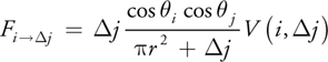
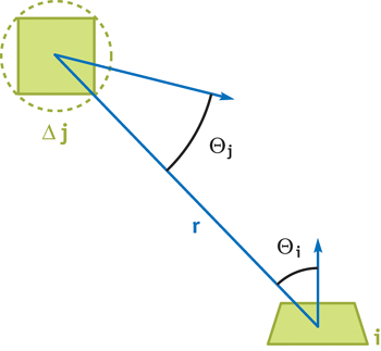
Figure 39-2 The Oriented-Disc Form Factor

39.1.1 Progressive Refinement

The classical radiosity algorithm (Goral et al. 1984) constructs and solves a large system of linear equations composed of the pairwise form factors. These equations describe the radiosity of an element as a function of the energy from every other element, weighted by their form factors and the element's reflectance, r. Thus the classical linear system requires O(N ²) storage, which is prohibitive for large scenes. The progressive refinement algorithm (Cohen et al. 1988) calculates these form factors on the fly, avoiding these storage requirements. It does this by repeatedly "shooting" out the energy from one element to all other elements in the scene.

Here's how progressive refinement works (Figure 39-3 illustrates two iterations of the algorithm). Each element in the scene maintains two energy values: an accumulated energy value and residual (or "unshot") energy. We choose one of the elements in the scene as the "shooter" and test the visibility of every other element from this shooter. If a receiving element is visible, then we calculate the amount of energy transferred from the shooter to the receiving element, as described by the corresponding form factor and the shooter's residual energy. This energy is multiplied by the receiver's reflectance, which is the fraction of incoming energy that is reflected back out again, and is usually represented by an RGB color. The resulting value is added to both the accumulated and the residual values of the receiving elements. Now that the shooter has cast out all of its energy, its residual energy is set to zero and the next shooter is selected. This process repeats until the residual energy of all of the elements has dropped below a threshold.

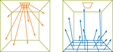
Figure 39-3 Two Iterations of the Progressive Refinement Solution

Initially, the residual energy of each light source element is set to a specified value and all other energy values are set to zero. After the first iteration, the scene polygon that has received the largest residual power (power = energy x area) is the next shooter. Selecting the largest residual power guarantees that the solution will converge rapidly (Cohen et al. 1988).

39.2 GPU Implementation

To implement this algorithm on the GPU, we use texels as radiosity elements (Heckbert 1990). There are two textures per scene polygon: a radiosity texture and a residual texture. Using textures as radiosity elements is similar to uniformly subdividing the scene, where the texture resolution determines the granularity of the radiosity solution.

If you sat down to implement progressive refinement radiosity, you might first try rendering the scene from the point of view of the shooter, and then "splatting" the energy into the textures of all of the visible polygons. This was our initial approach, and it had poor performance. The problem with this approach is that it requires the GPU to write to arbitrary locations in multiple textures. This type of "scatter" operation is difficult to implement on current graphics hardware.

Instead, we invert the computation by iterating over the receiving polygons and testing each element for visibility. This exploits the data-parallel nature of GPUs by executing the same small kernel program over many texels. This approach combines the high-quality reconstruction of gathering radiosity with the fast convergence and low storage requirements of shooting radiosity.

Each "shot" of the radiosity solution involves two passes: a visibility pass and a reconstruction pass. The visibility pass renders the scene from the point of view of the shooter and stores the scene in an item buffer. The reconstruction pass draws every potential receiving polygon orthographically into a frame buffer at the same resolution as the texture. This establishes a one-to-one correspondence between texels of the radiosity texture and fragments in the frame buffer. A fragment program tests the visibility and computes the analytic form factor. Pseudocode for our algorithm is shown in Listing 39-1. The next two sections describe the visibility and form factor computation in more detail.

Example 39-1. Pseudocode for Our Algorithm

initialize shooter residual E while not converged
{
render scene from POV of shooter
for each receiving element
{
  if element
    is visible
    {
      compute form factor FF E =
          *FF * E add E to residual texture add E to radiosity texture
    }
}
shooter's residual E = 0 compute next shooter
}

39.2.1 Visibility Using Hemispherical Projection

The visibility term of the form factor equation is usually computed using a hemicube (Cohen and Greenberg 1985), as shown in Figure 39-4. The scene is rendered onto the five faces of a cube map, which is then used to test visibility. Instead, we can avoid rendering the scene five times by using a vertex program to project the vertices onto a hemisphere. The hemispherical projection, also known as a stereographic projection, allows us to compute the visibility in only one rendering pass. The Cg code for this technique, which is similar to parabolic projection (Heidrich and Seidel 1998), is shown in Listing 39-2. Note that the z value is projected separately from the (x, y) position, which maintains the correct depth ordering and avoids precision issues.

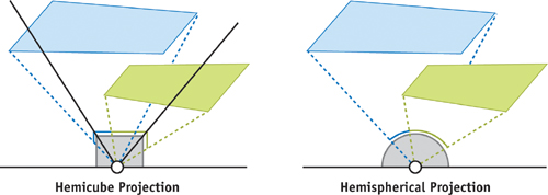
Figure 39-4 Hemicube and Hemispherical Projection

Example 39-2. Cg Code for Hemispherical Projection

void hemiwarp(float4 Position
              : POSITION, // pos in world space
                uniform half4x4 ModelView,
                // modelview matrix
                uniform half2 NearFar,
                // near and far planes
                out float4 ProjPos
              : POSITION)
// projected position
{
  // transform the geometry to camera space
  half4 mpos = mul(ModelView, Position);
  // project to a point on a unit hemisphere
  half3 hemi_pt = normalize(mpos.xyz);
  // Compute (f-n), but let the hardware divide z by this
  // in the w component (so premultiply x and y)
  half f_minus_n = NearFar.y - NearFar.x;
  ProjPos.xy = hemi_pt.xy * f_minus_n;
  // compute depth proj. independently, using OpenGL orthographic
  ProjPos.z = (-2.0 * mpos.z - NearFar.y - NearFar.x);
  ProjPos.w = f_minus_n;
}

The hemispherical projection vertex program calculates the positions of the projected elements, and the fragment program renders the unique ID of each element as color. Later, when we need to determine visibility, we use a fragment program to compare the ID of the receiver with the ID at the projected location in the item buffer. The Cg code for this lookup is shown in Listing 39-3.

Example 39-3. Cg Code for the Visibility Test

bool Visible(half3 ProjPos, // camera-space pos of element
             uniform fixed3 RecvID,
             // ID of receiver, for item buffer
             sampler2D HemiItemBuffer)
{
  // Project the texel element onto the hemisphere
  half3 proj = normalize(ProjPos);
  // Vector is in [-1,1], scale to [0..1] for texture lookup
  proj.xy = proj.xy * 0.5 + 0.5;
  // Look up projected point in hemisphere item buffer
  fixed3 xtex = tex2D(HemiItemBuffer, proj.xy);
  // Compare the value in item buffer to the ID of the fragment
  return all(xtex == RecvID);
}

This process is a lot like shadow mapping, except using polygon IDs rather than depth. Using the IDs avoids problems with depth precision, but it loses the advantages of the built-in shadow mapping hardware (such as percentage-closer filtering).

One drawback of hemispherical projection is that although polygon edges project to curves on a hemisphere, rasterization produces only straight edges. This is shown in Figure 39-5. To deal with this limitation, the scene polygons must be tessellated at a higher level of subdivision so that they can more closely approximate a curved edge.

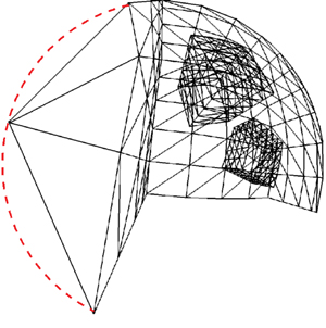
Figure 39-5 Rasterization Artifacts Caused by Insufficient Tessellation During Hemispherical Projection

39.2.2 Form Factor Computation

Once the visibility has been determined, we compute the energy transferred from the shooter to the receiver using the shooter-receiver form factor. This form factor computation is typically the most time-consuming part of the radiosity computation. We've implemented this in a fragment program in order to exploit the computational power of the fragment processor.

Listing 39-4 shows the code for the form factor computation, implemented in Cg.

Example 39-4. Cg Code for Form Factor Computation

half3 FormFactorEnergy(half3 RecvPos,
                       // world-space position of this element
                       uniform half3 ShootPos,
                       // world-space position of shooter
                       half3 RecvNormal,
                       // world-space normal of this element
                       uniform half3 ShootNormal,
                       // world-space normal of shooter
                       uniform half3 ShootEnergy,
                       // energy from shooter residual texture
                       uniform half ShootDArea,
                       // the delta area of the shooter
                       uniform fixed3 RecvColor)
// the reflectivity of this element
{
  // a normalized vector from shooter to receiver
  half3 r = ShootPos - RecvPos;
  half distance2 = dot(r, r);
  r = normalize(r);
  // the angles of the receiver and the shooter from r
  half cosi = dot(RecvNormal, r);
  half cosj = -dot(ShootNormal, r);
  // compute the disc approximation form factor
  const half pi = 3.1415926535;
  half Fij = max(cosi * cosj, 0) / (pi * distance2 + ShootDArea);
  Fij *= Visible();
  // returns visibility as 0 or 1
  // Modulate shooter's energy by the receiver's reflectivity
  // and the area of the shooter.
  half3 delta = ShooterEnergy * RecvColor * ShootDArea * Fij;
  return delta;
}

39.2.3 Choosing the Next Shooter

Progressive refinement techniques achieve fast convergence by shooting from the scene element with the highest residual power. To find the next shooter, we use a simple z-buffer sort. A mipmap pyramid is created from the residual texture of each element. The top level of this mipmap pyramid, which represents the average energy of the entire texture, is multiplied by the texture resolution to get the sum of the energy in the texture. Reductions of this sort are described in more detail in Buck and Purcell 2004 and Chapter 31 of this book, "Mapping Computational Concepts to GPUs."

This scalar value is multiplied by the area of the polygon, which gives us the total power of the polygon. We then draw a screen-aligned quadrilateral into a 1 x 1 frame buffer with the reciprocal of power as the depth and the unique polygon ID as the color. Each residual texture is rendered in this way, and z-buffering automatically selects the polygon with the highest power. We read back the 1-pixel frame buffer to get the ID of the next shooter. This technique also allows us to test convergence by setting the far clipping plane to the reciprocal of the convergence threshold. If no fragments are written, then the solution has converged.

39.3 Adaptive Subdivision

Until this point, we have been assuming that the radiosity textures are mapped one-to-one onto the scene geometry. This means that the scene is uniformly and statically tessellated (based on the texture resolution). However, uniform tessellation cannot adapt to the variable spatial frequency of the lighting. We would like to have more elements in areas of high-frequency lighting, such as shadow boundaries, and fewer elements in areas of low frequency, such as flat walls.

39.3.1 Texture Quadtree

A common technique for addressing these problems is to use an adaptive meshing solution (Heckbert 1990). Using this technique, we see that scene geometry is adaptively subdivided, with areas of higher lighting variation receiving a larger number of elements. In our system, each scene polygon acts as the root of a quadtree, and the radiosity data is stored in small (16x16) textures at the leaf nodes of the tree. This hierarchy can be thought of as a coarse adaptive geometric subdivision followed by a fine uniform texture subdivision. Figure 39-6 illustrates how a scene polygon can be subdivided into smaller quads based on the light variation.

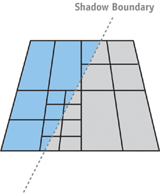
Figure 39-6 Quadtree Subdivision Adapts to the Frequency of the Lighting

Using this approach, we can reuse much of the code that we developed for the uniform case. The visibility and shooting are computed at each leaf node (instead of at each scene polygon), and the radiosity is reconstructed in a similar manner. The only difference is that as we compute the radiosity, we also must determine when to subdivide the quadtree.

39.3.2 Quadtree Subdivision

After every reconstruction pass, the leaf textures are evaluated for subdivision using a fragment program. There are several different techniques for determining when a quadtree node should be split. We use a technique that splits a node when the gradient of the radiosity exceeds a certain threshold (Vedel and Puech 1991). Using the gradient instead of the value avoids oversubdividing in areas where linear interpolation will adequately represent the function.

The gradient of the radiosity is evaluated in a fragment program, and fragments with gradient discontinuities are discarded. A hardware occlusion query is used to count these discarded fragments. If the number of discarded fragments exceeds our threshold, the current node is subdivided, and the process is repeated recursively. The recursion terminates when the radiosity is found to be smooth, or when a maximum depth is reached.

39.4 Performance

There are several optimization techniques for achieving interactive rates on small models. We use occlusion queries in the visibility pass to avoid reconstructing radiosity on surfaces that are not visible. We also shoot at a lower resolution than the texture resolution, which is called substructuring (Cohen et al. 1986). This can be done using the mipmaps that were created for the next-shooter selection.

If a polygon is selected as the next shooter, then all of the polygon's elements shoot their radiosity in turn. This amortizes the cost of mipmapping and sorting over multiple shots. We also batch together multiple shooters to reduce context switching.

Using these techniques, we've been able to compute a radiosity solution of a 10,000-element version of the Cornell Box scene to 90 percent convergence at about 2 frames per second.

For real-time applications, this technique can be combined with standard rendering techniques for higher performance. We can split the lighting into indirect and direct illumination by assuming that the indirect lighting is low frequency. This allows us to drastically reduce the texture resolution, which speeds up the calculation. The radiosity is calculated using the low-resolution textures, and the direct illumination is removed by setting the accumulated radiosity to zero after first iteration. The direct illumination is computed separately using lighting techniques such as per-pixel lighting and shadow volumes. The indirect illumination is added to this direct illumination to get the final image.

39.5 Conclusion

We've presented a method for implementing global illumination on graphics hardware by using progressive refinement radiosity. By exploiting the computational power of the fragment processor and rasterization hardware to compute the form factors, we can achieve interactive rates for scenes with a small number of elements (approximately 10,000). A scene with a large number of elements, such as that shown in Figure 39-7, can currently be rendered at noninteractive rates. As graphics hardware continues to increase in computational speed, we envision that global illumination will become a common part of lighting calculations.

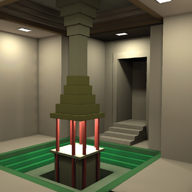
Figure 39-7 A Scene with One Million Elements Rendered with Our System

We use several GPU tricks to accelerate this algorithm, including the hemispherical projection and the z-buffer sort. These may have interesting applications beyond our implementation, such as environment mapping or penetration-depth estimation.

One of the limitations of radiosity is that it represents only diffuse surfaces. It would be interesting to try to extend this approach to nondiffuse surfaces. One approach could be to convolve the incoming lighting with an arbitrary BRDF and approximate the result with a low-coefficient polynomial or spherical harmonics (Sillion et al. 1991).

39.6 References

Buck, I., and T. Purcell. 2004. "A Toolkit for Computation on GPUs." In GPU Gems, edited by Randima Fernando, pp. 621–636. Addison-Wesley.

Cohen, M., S. E. Chen, J. R. Wallace, and D. P. Greenberg. 1988. "A Progressive Refinement Approach to Fast Radiosity Image Generation." In Computer Graphics (Proceedings of SIGGRAPH 88) 22(4), pp. 75–84.

Cohen, M., and D. P. Greenberg. 1985. "The Hemi-Cube: A Radiosity Solution for Complex Environments." In Computer Graphics (Proceedings of SIGGRAPH 85) 19(3), pp. 31–40.

Cohen, M., D. P. Greenberg, D. S. Immel, and P. J. Brock. 1986. "An Efficient Radiosity Approach for Realistic Image Synthesis." IEEE Computer Graphics and Applications 6(3), pp. 26–35.

Cohen, M., and J. Wallace. 1993. Radiosity and Realistic Image Synthesis. Morgan Kaufmann.

Goral, C. M., K. E. Torrance, D. P. Greenberg, and B. Battaile. 1984. "Modelling the Interaction of Light Between Diffuse Surfaces." In Computer Graphics (Proceedings of SIGGRAPH 84) 18(3), pp. 213–222.

Heckbert, P. 1990. "Adaptive Radiosity Textures for Bidirectional Ray Tracing." In Computer Graphics (Proceedings of SIGGRAPH 90) 24(4), pp. 145–154.

Heidrich, W., and H.-P. Seidel. 1998. "View-Independent Environment Maps." In Eurographics Workshop on Graphics Hardware 1998, pp. 39–45.

Sillion, F. X., J. R. Arvo, S. H. Westin, and D. P. Greenberg. 1991. "A Global Illumination Solution for General Reflectance Distributions." In Computer Graphics (Proceedings of SIGGRAPH 91) 25(4), pp. 187–196.

Vedel, C., and C. Puech. 1991. "A Testbed for Adaptive Subdivision in Progressive Radiosity." In Second Eurographics Workshop on Rendering.

Wallace, J. R., K. A. Elmquist, and E. A. Haines. 1989. "A Ray Tracing Algorithm for Progressive Radiosity." In Computer Graphics (Proceedings of SIGGRAPH 89) 23(4), pp. 315–324.

Copyright

Many of the designations used by manufacturers and sellers to distinguish their products are claimed as trademarks. Where those designations appear in this book, and Addison-Wesley was aware of a trademark claim, the designations have been printed with initial capital letters or in all capitals.

The authors and publisher have taken care in the preparation of this book, but make no expressed or implied warranty of any kind and assume no responsibility for errors or omissions. No liability is assumed for incidental or consequential damages in connection with or arising out of the use of the information or programs contained herein.

NVIDIA makes no warranty or representation that the techniques described herein are free from any Intellectual Property claims. The reader assumes all risk of any such claims based on his or her use of these techniques.

The publisher offers excellent discounts on this book when ordered in quantity for bulk purchases or special sales, which may include electronic versions and/or custom covers and content particular to your business, training goals, marketing focus, and branding interests. For more information, please contact:

U.S. Corporate and Government Sales
(800) 382-3419
corpsales@pearsontechgroup.com

For sales outside of the U.S., please contact:

International Sales
international@pearsoned.com

Visit Addison-Wesley on the Web: www.awprofessional.com

Library of Congress Cataloging-in-Publication Data

GPU gems 2 : programming techniques for high-performance graphics and general-purpose
computation / edited by Matt Pharr ; Randima Fernando, series editor.
p. cm.
Includes bibliographical references and index.
ISBN 0-321-33559-7 (hardcover : alk. paper)
1. Computer graphics. 2. Real-time programming. I. Pharr, Matt. II. Fernando, Randima.

T385.G688 2005
006.66—dc22
2004030181

GeForce™ and NVIDIA Quadro® are trademarks or registered trademarks of NVIDIA Corporation.

mental images and mental ray are trademarks or registered trademarks of mental images, GmbH.

All rights reserved. No part of this publication may be reproduced, stored in a retrieval system, or transmitted, in any form, or by any means, electronic, mechanical, photocopying, recording, or otherwise, without the prior consent of the publisher. Printed in the United States of America. Published simultaneously in Canada.

For information on obtaining permission for use of material from this work, please submit a written request to:

Pearson Education, Inc.
Rights and Contracts Department
One Lake Street
Upper Saddle River, NJ 07458

Text printed in the United States on recycled paper at Quebecor World Taunton in Taunton, Massachusetts.

Second printing, April 2005

Dedication

To everyone striving to make today's best computer graphics look primitive tomorrow