
GPU Gems 2
GPU Gems 2 is now available, right here, online. You can purchase a beautifully printed version of this book, and others in the series, at a 30% discount courtesy of InformIT and Addison-Wesley.
The CD content, including demos and content, is available on the web and for download.
Chapter 35. GPU Program Optimization
Cliff Woolley
University of Virginia
As GPU programmability has become more pervasive and GPU performance has become almost irresistibly appealing, increasing numbers of programmers have begun to recast applications of all sorts to make use of GPUs. But an interesting trend has appeared along the way: it seems that many programmers make the same performance mistakes in their GPU programs regardless of how much experience they have programming CPUs. The goal of this chapter is to help CPU programmers who are new to GPU programming avoid some of these common mistakes so that they gain the benefits of GPU performance without all the headaches of the GPU programmer's learning curve.
35.1 Data-Parallel Computing
One of the biggest hurdles you'll face when first programming a GPU is learning how to get the most out of a data-parallel computing environment. This parallelism exists at several levels on the GPU, as described in Chapter 29 of this book, "Streaming Architectures and Technology Trends." First, parallel execution on multiple data elements is a key design feature of modern GPUs. Vertex and fragment processors operate on four-vectors, performing four-component instructions such as additions, multiplications, multiply-accumulates, or dot products in a single cycle. They can schedule more than one of these instructions per cycle per pipeline. This provides ample opportunities for the extraction of instruction-level parallelism within a GPU program. For example, a series of sequential but independent scalar multiplications might be combined into a single four-component vector multiplication. Furthermore, parallelism can often be extracted by rearranging the data itself. For example, operations on a large array of scalar data will be inherently scalar. Packing the data in such a way that multiple identical scalar operations can occur simultaneously provides another means of exploiting the inherent parallelism of the GPU. (See Chapter 44 of this book, "A GPU Framework for Solving Systems of Linear Equations," for examples of this idea in practice.)
35.1.1 Instruction-Level Parallelism
While modern CPUs do have SIMD processing extensions such as MMX or SSE, most CPU programmers never attempt to use these capabilities themselves. Some count on the compiler to make use of SIMD extensions when possible; some ignore the extensions entirely. As a result, it's not uncommon to see new GPU programmers writing code that ineffectively utilizes vector arithmetic.
Let's take an example from a real-world application written by a first-time GPU programmer. In the following code snippet, we have a texture coordinate center and a uniform value called params. From them, a new coordinate offset is computed that will be used to look up values from the texture Operator:
float2 offset = float2(params.x * center.x - 0.5f * (params.x - 1.0f),
                       params.x *center.y - 0.5f * (params.x - 1.0f));
float4 O = f4texRECT(Operator, offset);
While the second line of this snippet (the actual texture lookup) is already as concise as possible, the first line leaves a lot to be desired. Each multiplication, addition, or subtraction is operating on a scalar value instead of a four-vector, wasting computational resources. Compilers for GPU programs are constantly getting better at detecting situations like this, but it's best to express arithmetic operations in vector form up front whenever possible. This helps the compiler do its job, and more important, it helps the programmer get into the habit of thinking in terms of vector arithmetic.
The importance of that habit becomes clearer when we look at the next snippet of code from that same fragment program. Here we take the center texture coordinate and use it to compute the coordinates of the four texels adjacent to center.
float4 neighbor =
    float4(center.x - 1.0f, center.x + 1.0f, center.y - 1.0f, center.y + 1.0f);
float output = (-O.x * f1texRECT(Source, float2(neighbor.x, center.y)) +
                -O.x * f1texRECT(Source, float2(neighbor.y, center.y)) +
                -O.y * f1texRECT(Source, float2(center.x, neighbor.z)) +
                -O.z * f1texRECT(Source, float2(center.x, neighbor.w))) /
               O.w;
Now not only have we made the mistake of expressing our additions and subtractions in scalar form, but we've also constructed from the four separate scalar results a four-vector neighbor that isn't even exactly what we need. To get the four texture coordinates we actually want, we have to assemble them one by one. That requires a number of move instructions. It would have been better to let the four-vector addition operation assemble the texture coordinates for us. The swizzle operator, discussed later in Section 35.2.4, helps here by letting us creatively rearrange the four-vector produced by the addition into multiple two-vector texture coordinates.
Performing the necessary manipulations to improve vectorization, here is an improved version of the preceding program:
float2 offset = center.xy - 0.5f;
offset = offset * params.xx + 0.5f; // multiply-and-accumulate
float4 x_neighbor = center.xyxy + float4(-1.0f, 0.0f, 1.0f, 0.0f);
float4 y_neighbor = center.xyxy + float4(0.0f, -1.0f, 0.0f, 1.0f);
float4 O = f4texRECT(Operator, offset);
float output = (-O.x * f1texRECT(Source, x_neighbor.xy) +
                -O.x * f1texRECT(Source, x_neighbor.zw) +
                -O.y * f1texRECT(Source, y_neighbor.xy) +
                -O.z * f1texRECT(Source, y_neighbor.zw)) /
               O.w;
An additional point of interest here is that the expression offset * params.xx + 0.5f, a multiply-and-accumulate operation, can be expressed as a single GPU assembly instruction and thus can execute in a single cycle. This allows us to achieve twice as many floating-point operations in the same amount of time.
Finally, notice that the output value could have been computed using a four-vector dot product. Unfortunately, while one of the two input vectors, O, is already on hand, the second one must be assembled from the results of four separate scalar texture lookups. Fortunately, the multiply-and-accumulate operation comes to the rescue once again in this instance. But in general, it seems wasteful to assemble four-vectors from scalar values just to get the benefit of a single vector operation. That's where data-level parallelism comes into play.
35.1.2 Data-Level Parallelism
Some problems are inherently scalar in nature and can be more effectively parallelized by operating on multiple data elements simultaneously. This data-level parallelism is particularly common in GPGPU applications, where textures and render targets are used to store large 2D arrays of scalar source data and output values. Packing the data more efficiently in such instances exposes the data-level parallelism. Of course, determining which packing of the data will be the most efficient requires a bit of creativity and is application-specific. Two common approaches are as follows:
- Split the data grid up into quadrants and stack the quadrants on top of each other by packing corresponding
scalar values into a single RGBA texel, as shown in Figure 35-1.
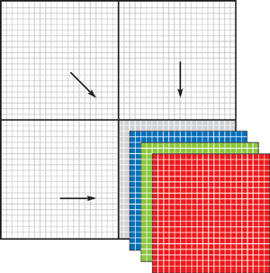
Figure 35-1 Packing Data by Stacking Grid Quadrants
- Take each group of four adjacent texels and pack them down into a single RGBA texel, as shown in Figure
35-2.
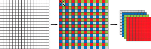
Figure 35-2 Packing Data by Stacking Adjacent Texels
There are ups and downs to each of these approaches, of course. While in theory there is a 4x speedup to be had by quartering the total number of fragments processed, the additional overhead of packing the data is significant in some cases, especially if the application requires the data to be unpacked again at the end of processing.
In some cases, application-specific data arrangements can be used to provide the speed of vector processing without the packing or unpacking overhead. For example, Goodnight et al. (2003a) use a data layout tailored to their application, which accelerates arbitrary-size separable convolutions on the GPU. Their approach trades off space for computation time by replicating the scalar data four times into the four channels for an RGBA texture, shifting the data by one texel in a given dimension per channel, as shown in Figure 35-3. Although this does not have the advantage of decreasing the number of fragments processed, it still leverages data-level parallelism by arranging data that will be used together in such a way that it can be accessed more efficiently, providing an overall speedup.
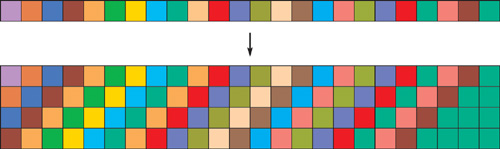
Figure 35-3 Custom Data Packing for Separable Convolutions
35.2 Computational Frequency
The next step in learning how to program GPUs effectively is learning to exploit the fact that the GPU comprises several different processors. Consider the typical rasterization pipeline. As implemented in hardware, the pipeline consists of a sequence of processors that operate in parallel and have different capabilities, degrees of programmability, strengths, and weaknesses. Between each stage of the pipeline is a work queue. Unless a pipeline stage's output work queue is full, that stage can work in parallel with other stages. While the CPU is busy handing off geometry and state information to the GPU, the GPU's vertex processor can process each vertex that arrives, transforming it and so forth. Simultaneously, the rasterizer can convert groups of transformed vertices into fragments (potentially many fragments), queuing them up for processing by the fragment processor.
Notice that the relative amount of work at each stage of the pipeline is typically increasing: a few vertices can result in the generation of many fragments, each of which can be expensive to process. Given this relative increase in the amount of work done at each stage, it is helpful to view the stages conceptually as a series of nested loops (even though each loop operates in parallel with the others, as just described). These conceptual nested loops work as shown in pseudocode in Listing 35-1.
Example 35-1. The Standard Rasterization Pipeline as a Series of Nested Loops
foreach
  tri in triangles
  {
    // run the vertex program on each vertex
    v1 = process_vertex(tri.vertex1);
    v2 = process_vertex(tri.vertex2);
    v3 = process_vertex(tri.vertex2);
    // assemble the vertices into a triangle
    assembledtriangle = setup_tri(v1, v2, v3);
    // rasterize the assembled triangle into [0..many] fragments
    fragments = rasterize(assembledtriangle);
    // run the fragment program on each fragment
    foreach
      frag in fragments { outbuffer[frag.position] = process_fragment(frag); }
  }
For each operation we perform, we must be mindful of how computationally expensive that operation is and how frequently it is performed. In a normal CPU program, this is fairly straightforward. With an actual series of nested loops (as opposed to the merely conceptual nested loops seen here), it's easy to see that a given expression inside an inner loop is loop-invariant and can be hoisted out to an outer loop and computed less frequently. Inner-loop branching in CPU programs is often avoided for similar reasons; the branch is expensive, and if it occurs in the inner loop, then it occurs frequently.
When writing GPU programs, it is particularly crucial to minimize the amount of redundant work. Naturally, all of the same techniques discussed previously for reducing computational frequency in CPU programs apply to GPU programs as well. But given the nature of GPU programming, each of the conceptual nested loops in Listing 35-1 is actually a separate program running on different hardware and possibly even written in different programming languages. That separation makes it easy to overlook some of these sorts of optimizations.
35.2.1 Precomputation of Loop Invariants
The first mistake a new GPU programmer is likely to make is to needlessly recompute values that vary linearly or are uniform across the geometric primitives inside a fragment program. Texture coordinates are a prime example. They vary linearly across the primitive being drawn, and the rasterizer interpolates them automatically. But when multiple related texture coordinates are used (such as the offset and neighbor coordinates in the example in Section 35.1.1), a common mistake is to compute the related values in the fragment program. This results in a possibly expensive computation being performed very frequently.
It would be much better to move the computation of the related texture coordinates into the vertex program. Though this effectively just shifts load around and interpolation in the rasterizer is still a per-fragment operation, the question is how much work is being done at each stage of the pipeline and how often that work must be done. Either way we do it, the result will be a set of texture coordinates that vary linearly across the primitive being drawn. But interpolation is often a lot less computationally expensive than recomputation of a given value on a per-fragment basis. As long as there are many more fragments than vertices, shifting the bulk of the computation so that it occurs on a per-vertex rather than a per-fragment basis makes sense.
It is worth reemphasizing, however, that any value that varies linearly across the domain can be computed in this way, regardless of whether it will eventually be used to index into a texture. Herein lies one of the keys to understanding GPU programming: the names that "special-purpose" GPU features go by are mostly irrelevant as long as you understand how they correspond to general-purpose concepts. Take a look at Chapter 31 of this book, "Mapping Computational Concepts to GPUs," for an in-depth look at those correspondences.
To take the concept of hoisting loop-invariant code a step further, some values are best precomputed on the CPU rather than on the GPU. Any value that is constant across the geometry being drawn can be factored all the way out to the CPU and passed to the GPU program as a uniform parameter. This sometimes results in parameters that are less than semantically elegant; for example, suppose we pass a uniform parameter size to a vertex or fragment program, but the program only uses the value size * size * 100. Although size and even size squared have semantic meaning, size squared times 100 has little. But again, if the GPU programs are equated to a series of nested loops and the goal is to remove redundant loop-invariant computations, it is likely still preferable to compute size * size * 100 on the CPU and pass that as the uniform parameter value to the GPU.
35.2.2 Precomputation Using Lookup Tables
In the more classic sense, "precomputation" means computation that is done offline in advance—the classic storage versus computation trade-off. This concept also maps readily onto GPUs: functions with a constant-size domain and range that are constant across runs of an algorithm—even if they vary in complex ways based on their input—can be precomputed and stored in texture maps.
Texture maps can be used for storing functions of one, two, or three variables over a finite domain as 1D, 2D, or 3D textures. Textures are usually indexed by floating-point texture coordinates between 0 and 1. The range is determined by the texture format used; 8-bit texture formats can only store values in the range [0, 1], but floating-point textures provide a much larger range of possible values. Textures can store up to four channels, so you can encode as many as four separate functions in the same texture. Texture lookups also provide filtering (interpolation), which you can use to get piecewise linear approximations to values in between the table entries.
As an example, suppose we had a fragment program that we wanted to apply to a checkerboard: half of the fragments of a big quad, the "red" ones, would be processed in one pass, while the other half, the "black" fragments, would be processed in a second pass. But how would the fragment program determine whether the fragment it was currently processing was red or black? One way would be to use modulo arithmetic on the fragment's position:
// Calculate red-black (odd-even) masks
float2 intpart;
float2 place = floor(1.0f - modf(round(position + 0.5f) / 2.0f, intpart));
float2 mask = float2((1.0f - place.x) * (1.0f - place.y), place.x *place.y);
if (((mask.x + mask.y) && do_red) || (!(mask.x + mask.y) && !do_red))
{
  // ...
}
Here, roughly speaking, place is the location of the fragment modulo 2 and mask.x and mask.y are Boolean values that together tell us whether the fragment is red or black. The uniform parameter do_red is set to 0 if we want to process the black fragments and 1 if we want the red fragments.
But clearly this is all a ridiculous amount of work for a seemingly simple task. It's much easier to precompute a checkerboard texture that stores a 0 in black texels and a 1 in red texels. Then we can skip all of the preceding arithmetic, replacing it with a single texture lookup, providing a substantial speedup. What we're left with is the following:
half4 mask = f4texRECT(RedBlack, IN.redblack);
/*
*
mask.x and mask.w tell whether IN.position.x and IN.position.y
*
are both odd or both even, respectively. Either of these two
*
conditions indicates that the fragment is red. params.x==1
*
selects red; params.y==1 selects black.
*/
if (dot(mask, params.xyyx))
{
  ...
}
However, although table lookups in this case were a win in terms of performance, that's not always going to be the case. Many GPU applications—particularly those that use a large number of four-component floating-point texture lookups—are memory-bandwidth-limited, so the introduction of an additional texture read in order to save a small amount of computation might in fact be a loss rather than a win. Furthermore, texture cache coherence is critical; a lookup table that is accessed incoherently will thrash the cache and hurt performance rather than help it. But if enough computation can be "pre-baked" or if the GPU programs in question are compute-limited already, and if the baked results are read from the texture in a spatially coherent way, table lookups can improve performance substantially. See Section 35.3 later in this chapter for more on benchmarking and GPU application profiling.
35.2.3 Avoid Inner-Loop Branching
In CPU programming, it is often desirable to avoid branching inside inner loops. This usually involves making several copies of the loop, with each copy acting on a subset of the data and following the execution path specific to that subset. This technique is sometimes called static branch resolution or substreaming.
The same concept applies to GPUs. Because a fragment program conceptually represents an inner loop, applying this technique requires a fragment program containing a branch to be divided into multiple fragment programs without the branch. The resulting programs each account for one code execution path through the original, monolithic program. This technique also requires the application to subdivide the data, which for the GPU means rasterization of multiple primitives instead of one. See Chapter 34 of this book, "GPU Flow-Control Idioms," for details.
A typical example is a 2D grid where data elements on the boundary of the grid require special handling that does not apply to interior elements. In this case, it is preferable to create two separate fragment programs—a short one that does not account for boundary conditions and a longer one that does—and draw a filled-in quad over the interior elements and an outline quad over the boundary elements.
35.2.4 The Swizzle Operator
An easily overlooked or underutilized feature of GPU programming is the swizzle operator. Because all registers on the GPU are four-vectors but not all instructions take four-vectors as arguments, some mechanism for creating other-sized vectors out of these four-vector registers is necessary. The swizzle operator provides this functionality. It is syntactically similar to the C concept of a structure member access but has the additional interesting property that data members can be rearranged, duplicated, or omitted in arbitrary combinations, as shown in the following example:
float4 f = float4(1.0f, 2.0f, 3.0f, 4.0f);
float4 g = float4(5.0f, 6.0f, 7.0f, 8.0f);
float4 h = float4(0.1f, 0.2f, 0.3f, 0.4f);
// note that h.w is syntactically equivalent to h.wwww
float4 out = f.xyyz * g.wyxz + h.w; // this is one instruction!
                                    // multiply-and-accumulate again.
// result: out is (8.4f, 12.4f, 10.4f, 21.4f)
The swizzle operator has applications in the computational frequency realm. For example, consider the common case of a fragment program that reads from three adjacent texels: (x, y), (x - 1, y), and (x + 1, y). Computing the second and third texture coordinates from the first is a job best left to the vertex program and rasterizer, as has already been discussed. But the rasterizer can interpolate four-vectors as easily as it can two-vectors, so there is no reason that these three texture coordinates should have to occupy three separate interpolants. In fact, there are only four distinct values being used: x, x - 1, x + 1, and y. So all three texture coordinates can actually be packed into and interpolated as a single four-vector. The three distinct two-vector texture coordinates are simply extracted (for free) from the single four-vector interpolant in the fragment program by using swizzle operators, as shown here:
struct vertdata
{
  float4 position : POSITION;
  float4 texcoord : TEXCOORD0;
} vertdata vertexprog(vertdata IN)
{
  vertdata OUT;
  OUT.position = IN.position;
  OUT.texcoord = float4(IN.texcoord.x, IN.texcoord.y, IN.texcoord.x - 1,
                        IN.texcoord.x + 1);
  return vertdata;
}
frag2frame fragmentprog(vertdata IN, uniform samplerRECT texmap)
{
  ... float4 center = f4texRECT(texmap, IN.texcoord.xy);
  float4 left = f4texRECT(texmap, IN.texcoord.zy);
  float4 right = f4texRECT(texmap, IN.texcoord.wy);
  ...
}
Not only does this save on arithmetic in the vertex processor, but it saves interpolants as well. Further, it avoids the construction of vectors in the fragment program: swizzles are free (on NVIDIA GeForce FX and GeForce 6 Series GPUs), but the move instructions required to construct vectors one channel at a time are not. We saw this same issue in Section 35.1.1.
Also worth mentioning is a syntactic cousin of the swizzle operator: the write mask operator. The write mask specifies a subset of the destination variable's components that should be modified by the current instruction. This can be used as a hint to the compiler that unnecessary work can be avoided. For example, if a write mask is applied to a texture lookup, memory bandwidth could be saved because texture data in channels that will never be used need not be read from texture memory. Note that although the syntax of a write mask is similar to that of a swizzle, the concepts of rearranging or duplicating channels do not apply to a write mask.
float4 out;
out = float4(1.0f, 2.0f, 3.0f, 4.0f);
out.xz = float4(5.0f, 6.0f, 7.0f, 8.0f);
// result: out is (5.0f, 2.0f, 7.0f, 4.0f)
35.3 Profiling and Load Balancing
As with CPU programming, the best way to write efficient GPU code is to write something straightforward that works and then optimize it iteratively as necessary. Unfortunately, this process currently isn't quite as easy with GPU code, because fewer tools exist to help with it. But a bit of extra diligence on the part of the programmer allows optimization to be done effectively even in the absence of special tools.
Frequent timing measurements are the key. In fact, every optimization that gets applied should be independently verified by timing it. Even optimizations that seem obvious and certain to result in a speedup can in fact provide no gain at all or, worse, cause a slowdown. When this happens, it might indicate a load imbalance in the graphics pipeline, but such problems can also arise because the final optimization step occurs inside the graphics driver, making it difficult for the programmer to know exactly what code is really being executed. A transformation made on the source code that seems beneficial might in fact disable some other optimization being done by the driver, causing a net loss in performance. These sorts of problems are much more easily detected by benchmarking after each optimization; backtracking to isolate problematic optimizations after the fact is a waste of time and energy.
Once the obvious optimizations have been applied, a low-level understanding of the capabilities of the hardware, particularly in terms of superscalar instruction issues, becomes useful. The more detailed your knowledge of what kinds of instructions can be executed simultaneously, the more likely you will be to recognize additional opportunities for code transformation and improvement. The NVShaderPerf tool helps with this by showing you exactly how your fragment programs schedule onto the arithmetic units of the GPU, taking much of the guesswork out of fragment program optimization. (For more information on NVShaderPerf, see "References" at the end of the chapter.)
Even with the most highly tuned fragment programs imaginable, there's still a chance that a GPU application can be made to run faster. At this point it becomes a matter of finding the main bottleneck in the application and shifting load away from it as much as possible. The first step is to use a CPU-application profiling tool, such as Rational Quantify, Intel VTune, or AMD CodeAnalyst. This can help pinpoint problems like driver overhead (such as in context switching). Not all of the information that such a profiler provides will be reliable; many graphics API calls are nonblocking so that the CPU and GPU can operate in parallel. At some point, the GPU's work queue will fill up and an arbitrary API call on the CPU side will block to wait for the GPU to catch up. The blocked call will be counted by the CPU profiler as having taken a long time to execute, even if the work done during that time would be more fairly attributed to an earlier API call that did not block. As long as this caveat is kept in mind, however, CPU profilers can still provide valuable insights.
Once CPU overhead is minimized, the only remaining issue is determining where the GPU bottlenecks lie. Specialized tools for monitoring GPU performance are beginning to appear on the market for this purpose; NVPerfHUD is a good example (see "References" for more on NVPerfHUD). To the extent that these tools do not yet provide detailed information or are inapplicable to a particular application (NVPerfHUD, for example, is currently Direct3D-only and is not well suited to GPGPU applications), other techniques can be utilized to fill in the gaps. Each involves a series of experiments. One approach is to test whether the addition of work to a given part of the GPU pipeline increases the total execution time or the reduction of work decreases execution time. If so, it's likely that that is where the main bottleneck lies. For example, if a fragment program is compute-limited, then inserting additional computation instructions will increase the time it takes the program to execute; but if the program is memory-bandwidth-limited, the extra computation can probably be done for free. An alternate approach is to underclock either the compute core or the memory system of the graphics card. If the memory system can be underclocked without decreasing performance, then memory bandwidth is not the limiting factor. These techniques and many more are detailed in the NVIDIA GPU Programming Guide (NVIDIA 2004).
Ultimately, understanding the bottlenecks is the key to knowing how to get them to go away. A combination of the preceding techniques and a bit of experience will aid in that understanding.
35.4 Conclusion
As we've seen, GPU program optimization shares many common themes with CPU program optimization. High-level languages for GPGPU that provide a unified stream programming model (and thus, hopefully, more opportunities for global GPU application optimization) are emerging (McCool et al. 2002, Buck et al. 2004), and automatic optimization of GPU code is constantly improving. But until those technologies have matured, GPU programmers will continue to have to take responsibility for high-level optimizations and understand the details of the hardware they're working with to get the most out of low-level optimizations. Hopefully this chapter has given you the tools you need to learn how best to extract from your GPU application all of the performance that the GPU has to offer.
35.5 References
Buck, Ian, Tim Foley, Daniel Horn, Jeremy Sugerman, Kayvon Fatahalian, Mike Houston, and Pat Hanrahan. 2004. "Brook for GPUs: Stream Computing on Graphics Hardware." ACM Transactions on Graphics (Proceedings of SIGGRAPH 2004) 23(3), pp. 777–786. Available online at http://graphics.stanford.edu/projects/brookgpu/
Goodnight, Nolan, Rui Wang, Cliff Woolley, and Greg Humphreys. 2003a. "Interactive Time-Dependent Tone Mapping Using Programmable Graphics Hardware." In Eurographics Symposium on Rendering: 14th Eurographics Workshop on Rendering, pp. 26–37.
Goodnight, Nolan, Cliff Woolley, Gregory Lewin, David Luebke, and Greg Humphreys. 2003b. "A Multigrid Solver for Boundary Value Problems Using Programmable Graphics Hardware." In Proceedings of the SIGGRAPH/Eurographics Workshop on Graphics Hardware 2003, pp. 102–111.
McCool, Michael D., Zheng Qin, and Tiberiu S. Popa. 2002. "Shader Metaprogramming." In Proceedings of the SIGGRAPH/Eurographics Workshop on Graphics Hardware 2002, pp. 57–68. Revised article available online at http://www.cgl.uwaterloo.ca/Projects/rendering/Papers/index.html#metaprog
NVIDIA. 2004. NVIDIA GPU Programming Guide. Available online at http://developer.nvidia.com/object/gpu_programming_guide.html
NVPerfHUD. Available online at http://developer.nvidia.com/object/nvperfhud_home.html
NVShaderPerf. Available online at http://developer.nvidia.com/object/nvshaderperf_home.html
Copyright
Many of the designations used by manufacturers and sellers to distinguish their products are claimed as trademarks. Where those designations appear in this book, and Addison-Wesley was aware of a trademark claim, the designations have been printed with initial capital letters or in all capitals.
The authors and publisher have taken care in the preparation of this book, but make no expressed or implied warranty of any kind and assume no responsibility for errors or omissions. No liability is assumed for incidental or consequential damages in connection with or arising out of the use of the information or programs contained herein.
NVIDIA makes no warranty or representation that the techniques described herein are free from any Intellectual Property claims. The reader assumes all risk of any such claims based on his or her use of these techniques.
The publisher offers excellent discounts on this book when ordered in quantity for bulk purchases or special sales, which may include electronic versions and/or custom covers and content particular to your business, training goals, marketing focus, and branding interests. For more information, please contact:
U.S. Corporate and Government Sales
(800) 382-3419
corpsales@pearsontechgroup.com
For sales outside of the U.S., please contact:
International Sales
international@pearsoned.com
Visit Addison-Wesley on the Web: www.awprofessional.com
Library of Congress Cataloging-in-Publication Data
GPU gems 2 : programming techniques for high-performance graphics and general-purpose
computation / edited by Matt Pharr ; Randima Fernando, series editor.
p. cm.
Includes bibliographical references and index.
ISBN 0-321-33559-7 (hardcover : alk. paper)
1. Computer graphics. 2. Real-time programming. I. Pharr, Matt. II. Fernando, Randima.
T385.G688 2005
006.66—dc22
2004030181
GeForce™ and NVIDIA Quadro® are trademarks or registered trademarks of NVIDIA Corporation.
Nalu, Timbury, and Clear Sailing images © 2004 NVIDIA Corporation.
mental images and mental ray are trademarks or registered trademarks of mental images, GmbH.
Copyright © 2005 by NVIDIA Corporation.
All rights reserved. No part of this publication may be reproduced, stored in a retrieval system, or transmitted, in any form, or by any means, electronic, mechanical, photocopying, recording, or otherwise, without the prior consent of the publisher. Printed in the United States of America. Published simultaneously in Canada.
For information on obtaining permission for use of material from this work, please submit a written request to:
Pearson Education, Inc.
Rights and Contracts Department
One Lake Street
Upper Saddle River, NJ 07458
Text printed in the United States on recycled paper at Quebecor World Taunton in Taunton, Massachusetts.
Second printing, April 2005
Dedication
To everyone striving to make today's best computer graphics look primitive tomorrow
- Copyright
- Inside Back Cover
- Inside Front Cover
- Part I: Geometric Complexity
-
- Chapter 1. Toward Photorealism in Virtual Botany
- Chapter 2. Terrain Rendering Using GPU-Based Geometry Clipmaps
- Chapter 3. Inside Geometry Instancing
- Chapter 4. Segment Buffering
- Chapter 5. Optimizing Resource Management with Multistreaming
- Chapter 6. Hardware Occlusion Queries Made Useful
- Chapter 7. Adaptive Tessellation of Subdivision Surfaces with Displacement Mapping
- Chapter 8. Per-Pixel Displacement Mapping with Distance Functions
- Part II: Shading, Lighting, and Shadows
-
- Chapter 9. Deferred Shading in S.T.A.L.K.E.R.
- Chapter 10. Real-Time Computation of Dynamic Irradiance Environment Maps
- Chapter 11. Approximate Bidirectional Texture Functions
- Chapter 12. Tile-Based Texture Mapping
- Chapter 13. Implementing the mental images Phenomena Renderer on the GPU
- Chapter 14. Dynamic Ambient Occlusion and Indirect Lighting
- Chapter 15. Blueprint Rendering and "Sketchy Drawings"
- Chapter 16. Accurate Atmospheric Scattering
- Chapter 17. Efficient Soft-Edged Shadows Using Pixel Shader Branching
- Chapter 18. Using Vertex Texture Displacement for Realistic Water Rendering
- Chapter 19. Generic Refraction Simulation
- Part III: High-Quality Rendering
-
- Chapter 20. Fast Third-Order Texture Filtering
- Chapter 21. High-Quality Antialiased Rasterization
- Chapter 22. Fast Prefiltered Lines
- Chapter 23. Hair Animation and Rendering in the Nalu Demo
- Chapter 24. Using Lookup Tables to Accelerate Color Transformations
- Chapter 25. GPU Image Processing in Apple's Motion
- Chapter 26. Implementing Improved Perlin Noise
- Chapter 27. Advanced High-Quality Filtering
- Chapter 28. Mipmap-Level Measurement
- Part IV: General-Purpose Computation on GPUS: A Primer
-
- Chapter 29. Streaming Architectures and Technology Trends
- Chapter 30. The GeForce 6 Series GPU Architecture
- Chapter 31. Mapping Computational Concepts to GPUs
- Chapter 32. Taking the Plunge into GPU Computing
- Chapter 33. Implementing Efficient Parallel Data Structures on GPUs
- Chapter 34. GPU Flow-Control Idioms
- Chapter 35. GPU Program Optimization
- Chapter 36. Stream Reduction Operations for GPGPU Applications
- Part V: Image-Oriented Computing
-
- Chapter 37. Octree Textures on the GPU
- Chapter 38. High-Quality Global Illumination Rendering Using Rasterization
- Chapter 39. Global Illumination Using Progressive Refinement Radiosity
- Chapter 40. Computer Vision on the GPU
- Chapter 41. Deferred Filtering: Rendering from Difficult Data Formats
- Chapter 42. Conservative Rasterization
- Part VI: Simulation and Numerical Algorithms
-
- Chapter 43. GPU Computing for Protein Structure Prediction
- Chapter 44. A GPU Framework for Solving Systems of Linear Equations
- Chapter 45. Options Pricing on the GPU
- Chapter 46. Improved GPU Sorting
- Chapter 47. Flow Simulation with Complex Boundaries
- Chapter 48. Medical Image Reconstruction with the FFT