
GPU Gems 2
GPU Gems 2 is now available, right here, online. You can purchase a beautifully printed version of this book, and others in the series, at a 30% discount courtesy of InformIT and Addison-Wesley.
The CD content, including demos and content, is available on the web and for download.
Chapter 2. Terrain Rendering Using GPU-Based Geometry Clipmaps
Arul Asirvatham
Microsoft Research
Hugues Hoppe
Microsoft Research
The geometry clipmap introduced in Losasso and Hoppe 2004 is a new level-of-detail structure for rendering terrains. It caches terrain geometry in a set of nested regular grids, which are incrementally shifted as the viewer moves. The grid structure provides a number of benefits over previous irregular-mesh techniques: simplicity of data structures, smooth visual transitions, steady rendering rate, graceful degradation, efficient compression, and runtime detail synthesis. In this chapter, we describe a GPU-based implementation of geometry clipmaps, enabled by vertex textures. By processing terrain geometry as a set of images, we can perform nearly all computations on the GPU itself, thereby reducing CPU load. The technique is easy to implement, and allows interactive flight over a 20-billion-sample grid of the United States stored in just 355 MB of memory, at around 90 frames per second.
2.1 Review of Geometry Clipmaps
In large outdoor environments, the geometry of terrain landscapes can require significant storage and rendering bandwidth. Numerous level-of-detail techniques have been developed to adapt the triangulation of the terrain mesh as a function of the view. However, most such techniques involve runtime creation and modification of mesh structures (vertex and index buffers), which can prove expensive on current graphics architectures. Moreover, use of irregular meshes generally requires processing by the CPU, and many applications such as games are already CPU-limited.
The geometry clipmap framework (Losasso and Hoppe 2004) treats the terrain as a 2D elevation image, prefiltering it into a mipmap pyramid of L levels as illustrated in Figure 2-1. For complex terrains, the full pyramid is too large to fit in memory. The geometry clipmap structure caches a square window of nxn samples within each level, much like the texture clipmaps of Tanner et al. 1998. These windows correspond to a set of nested regular grids centered about the viewer, as shown in Figure 2-2. Note that the finer-level windows have smaller spatial extent than the coarser ones. The aim is to maintain triangles that are uniformly sized in screen space. With a clipmap size n = 255, the triangles are approximately 5 pixels wide in a 1024x768 window.
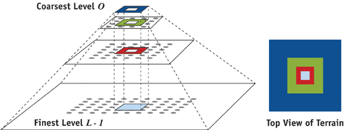
Figure 2-1 How Geometry Clipmaps Work
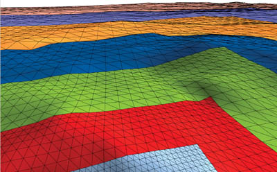
Figure 2-2 Terrain Rendering Using a Coarse Geometry Clipmap
Only the finest level is rendered as a complete grid square. In all other levels, we render a hollow "ring," which omits the interior region already rendered at finer resolutions.
As the viewer moves, the clipmap windows are shifted and updated with new data. To permit efficient incremental updates, the clipmap window in each level is accessed toroidally, that is, with 2D wraparound addressing (see Section 2.4).
One of the challenges with the clipmap structure is to hide the boundaries between successive resolution levels, while at the same time maintaining a watertight mesh and avoiding temporal popping artifacts. The nested grid structure of the geometry clipmap provides a simple solution. The key idea is to introduce a transition region near the outer perimeter of each level, whereby the geometry and textures are smoothly morphed to interpolate the next-coarser level (see Figure 2-3). These transitions are efficiently implemented in the vertex and pixel shaders, respectively.
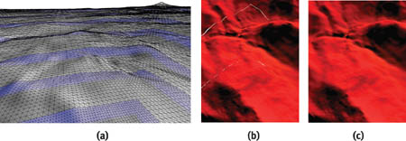
Figure 2-3 Achieving Visual Continuity by Blending Within Transition Regions
The nested grid structure of the geometry clipmap also enables effective compression and synthesis. It allows the prediction of the elevation data for each level by upsampling the data from the coarser level. Thus, one need only store or synthesize the residual detail added to this predicted signal.
2.2 Overview of GPU Implementation
The original implementation of geometry clipmaps presented in Losasso and Hoppe 2004 represents each clipmap level as a traditional vertex buffer. Because the GPU currently lacks the ability to modify vertex buffers, that implementation required significant intervention by the CPU to both update and render the clipmap (see Table 2-1).
Table 2-1. Comparison with Original CPU Implementation
|
Our implementation of geometry clipmaps using vertex textures moves nearly all operations to the GPU. |
||
|
Original Implementation [1] |
GPU-Based Implementation |
|
|
Elevation Data |
In vertex buffer |
In 2D vertex texture |
|
Vertex Buffer |
Incrementally updated by CPU |
Constant! |
|
Index Buffer |
Generated every frame by CPU |
Constant! |
|
Upsampling |
CPU |
GPU |
|
Decompression |
CPU |
CPU |
|
Synthesis |
CPU |
GPU |
|
Adding Residuals |
CPU |
GPU |
|
Normal-Map Update |
CPU |
GPU |
|
Transition Blends |
GPU |
GPU |
In this chapter, we describe an implementation of geometry clipmaps using vertex textures. This is advantageous because the 2D grid data of each clipmap window is much more naturally stored as a 2D texture, rather than being artificially linearized into a 1D vertex buffer.
Recall that the clipmap has L levels, each containing a grid of nxn geometric samples. Our approach is to split the (x, y, z) geometry of the samples into two parts:
- The (x, y) coordinates are stored as constant vertex data.
- The z coordinate is stored as a single-channel 2D texture—the elevation map. We define a separate nxn elevation map texture for each clipmap level. These textures are updated as the clipmap levels shift with the viewer's motion.
Because clipmap levels are uniform 2D grids, their (x, y) coordinates are regular, and thus constant up to a translation and scale. Therefore, we define a small set of read-only vertex and index buffers, which describe 2D "footprints," and repeatedly instance these footprints both within and across resolution levels, as described in Section 2.3.2.
The vertices obtain their z elevations by sampling the elevation map as a vertex texture. Accessing a texture in the vertex shader is a new feature in DirectX 9 Shader Model 3.0, and is supported by GPUs such as the NVIDIA GeForce 6 Series.
Storing the elevation data as a set of images allows direct processing using the GPU rasterization pipeline (as noted in Table 2-1). For the case of synthesized terrains, all runtime computations (elevation-map upsampling, terrain detail synthesis, normal-map computation, and rendering) are performed entirely within the graphics card, leaving the CPU basically idle. For compressed terrains, the CPU incrementally decompresses and uploads data to the graphics card (see Section 2.4).
2.2.1 Data Structures
To summarize, the main data structures are as follows. We predefine a small set of constant vertex and index buffers to encode the (x, y) geometry of the clipmap grids. And for each level 0 . . . L–1, we allocate an elevation map (a 1-channel floating-point 2D texture) and a normal map (a 4-channel 8-bit 2D texture). All these data structures reside in video memory.
2.2.2 Clipmap Size
Because the outer perimeter of each level must lie on the grid of the next-coarser level (as shown in Figure 2-4), the grid size n must be odd. Hardware may be optimized for texture sizes that are powers of 2, so we choose n = 2 k -1 (that is, 1 less than a power of 2) leaving 1 row and 1 column of the textures unused. Most of our examples use n = 255.
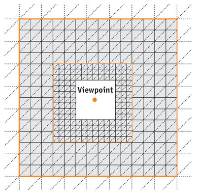
Figure 2-4 Two Successive Clipmap Rings
The choice of grid size n = 2 k -1 has the further advantage that the finer level is never exactly centered with respect to its parent next-coarser level. In other words, it is always offset by 1 grid unit either left or right, as well as either top or bottom (see Figure 2-4), depending on the position of the viewpoint. In fact, it is necessary to allow a finer level to shift while its next-coarser level stays fixed, and therefore the finer level must sometimes be off-center with respect to the next-coarser level. An alternative choice of grid size, such as n = 2 k -3, would provide the possibility for exact centering, but it would still require the handling of off-center cases and thus result in greater overall complexity.
2.3 Rendering
2.3.1 Active Levels
Although we have allocated L levels for the clipmap, we often render (and update) only a set of active levels 0 . . . L'-1, where the number of levels L'  L is based on the height of the viewpoint over the underlying terrain. The motivation is that when the viewer is sufficiently high, the finest clipmap levels are unnecessarily dense and in fact result in aliasing artifacts. Specifically, we deactivate levels for which the grid extent is smaller than 2.5h, where h is the viewer height above the terrain. Since all the terrain data resides in video memory, computing h involves reading back one point sample (immediately below the viewpoint) from the elevation map texture of the finest active level (L'-1). This readback incurs a small cost, so we perform it only every few frames. Of course, we render level L'-1 using a complete square rather than a hollow ring.
The implementation described in Losasso and Hoppe 2004 allows "cropping" of a level if its data was not fully updated during viewer motion. To simplify our GPU implementation, we have decided to forgo this feature. We instead assume that a level is either fully updated or declared inactive.
2.3.2 Vertex and Index Buffers
As explained earlier, we represent the grid (x, y) values as vertex data, while storing the z elevation values as a one-channel floating-point texture. A brute-force approach would be to define a single vertex buffer containing the (x, y) data for the entire ring within a level. To both reduce memory costs and enable view frustum culling, we instead break the ring into smaller 2D footprint pieces, as illustrated in Figure 2-5.
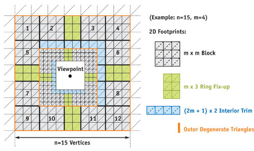
Figure 2-5 Partitioning a Clipmap Ring
Most of the ring is created using 12 blocks (shown in gray) of size mxm, where m = (n + 1)/4. Since the 2D grid is regular, the (x, y) geometries of all blocks within a level are identical up to a translation. Moreover, they are also identical across levels up to a uniform scale. Therefore, we can render the (x, y) geometries of all terrain blocks using a single read-only vertex buffer and index buffer, by letting the vertex shader scale and translate the block (x, y) geometry using a few parameters.
For our default clipmap size n = 255, this canonical block has 64x64 vertices. The index buffer encodes a set of indexed triangle strips whose lengths are chosen for optimal vertex caching. We use 16-bit indices for the index buffer, which allows a maximum block size of m = 256 and therefore a maximum clipmap size of n = 1023.
However, the union of the 12 blocks does not completely cover the ring. We fill the small remaining gaps using a few additional 2D footprints, as explained next. Note that in practice, these additional regions have a very small area compared to the regular mxm blocks, as revealed in Figure 2-6. First, there is a gap of (n -1) - ((m -1) x 4) = 2 quads at the middle of each ring side. We patch these gaps using four mx3 fix-up regions (shown in green in Figures 2-5 and 2-6). We encode these regions using one vertex and index buffer, and we reuse these buffers across all levels. Second, there is a gap of one quad on two sides of the interior ring perimeter, to accommodate the off-center finer level. This L-shaped strip (shown in blue) can lie at any of four possible locations (top-left, top-right, bottom-left, bottom-right), depending on the relative position of the fine level inside the coarse level. We define four vertex and one index buffer for this interior trim, and we reuse these across all levels.
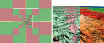
Figure 2-6 Visualizing the Nested Grid Structure
Also, we render a string of degenerate triangles (shown in orange) on the outer perimeter. These zero-area triangles are necessary to avoid mesh T-junctions. Finally, for the finest level, we fill the ring interior with four additional blocks and one more L-shaped region.
Because the footprint (x, y) coordinates are local, these do not require 32-bit precision, so we pack them into a D3DDECLTYPE_SHORT2, requiring only 4 bytes per vertex. In the future, it may be possible to compute the (x, y) coordinates within the mxm block from the vertex index i itself as (fmod(i, m), floor(i/m)).
2.3.3 View Frustum Culling
View frustum culling is done at the block level on the CPU. Each block is extruded by [z min, z max] and intersected with the view frustum in 3D. It is rendered only if this intersection is nonempty. Depending on the view direction, the rendering load is reduced by a factor of 2 to 3 for a 90-degree field of view, as shown in Figure 2-7.
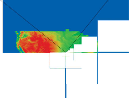
Figure 2-7 View Frustum Culling
2.3.4 DrawPrimitive Calls
For each level, we make up to 14 DrawPrimitive (DP) calls: 12 for the blocks, 1 for the interior trim, and 1 for the remaining triangles. With view frustum culling, on average only 4 of the 12 blocks are rendered each frame. The finest level requires 5 more calls to fill the interior hole. Thus, overall we make 6L + 5 (71 for L = 11) DP calls per frame on average. This total number could be further reduced to 3L + 2 (35) by instancing all blocks rendered in each level using a single DP call.
2.3.5 The Vertex Shader
The same vertex shader is applied to the rendering of all 2D footprints described previously. First, given the footprint (x, y) coordinates, the shader computes the world (x, y) coordinates using a simple scaling and translation. Next, it reads the z value from the elevation map stored in the vertex texture. No texture filtering is necessary because the vertices correspond one-to-one with the texture samples.
For smooth transitions, the vertex shader blends the geometry near the outer boundary of each level with that of the next-coarser level. It computes the blending parameter based on the (x, y) location relative to the continuous viewer position (v x , v y ). Specifically, = max( x , y ), with
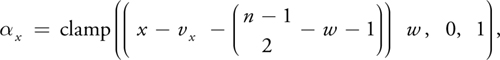
and similarly for y .
Here, all coordinates are expressed in the [0 . . . n-1] range of the clipmap grid, and w is the transition width (chosen to be n/10). The desired property is that evaluates to 0 except in the transition region, where it ramps up linearly to reach 1 at the outer perimeter. Figure 2-3a (on page 29) shows the evaluation of the parameter within the transition regions in purple.
For geometric blending, we linearly interpolate between the current (fine-level) elevation z f and the elevation z c at the same (x, y) location in the next-coarser level:
|
z' = (1 - ) zf + zc |
In the general case, the sample location lies on an edge of the coarser grid, and z c is obtained by averaging the two coarse samples on the edge endpoints. We could perform this computation at runtime, but it would require a total of three vertex-texture lookups (one for z f and two for z c = (z c 1 + z c 2)/2) and vertex-texture reads are currently expensive (Gerasimov et al. 2004).
Instead, we compute z c as part of the clipmap update, and pack both z f and z c into the same 1-channel floating-point texture. We achieve this by storing z f into the integer part of the float, and the difference z d = z c - z f (scaled) into the fractional part. The packing is done in the pixel shader of the upsampling stage (see Section 2.4.1).
Listing 2-1 is the High-Level Shader Language (HLSL) vertex program for clipmap rendering.
Example 2-1. Vertex Shader Code for Rendering a Clipmap Level
struct OUTPUT
{
  vector pos : POSITION;
  float2 uv : TEXCOORD0;
  // coordinates for normal-map lookup
  float z : TEXCOORD1;
  // coordinates for elevation-map lookup
  float alpha : TEXCOORD2; // transition blend on normal map
};
uniform float4 ScaleFactor, FineBlockOrig;
uniform float2 ViewerPos, AlphaOffset, OneOverWidth;
uniform float ZScaleFactor, ZTexScaleFactor;
uniform matrix WorldViewProjMatrix;
// Vertex shader for rendering the geometry clipmap
OUTPUT RenderVS(float2 gridPos : TEXCOORD0)
{
  OUTPUT output;
  // convert from grid xy to world xy coordinates
  //
  ScaleFactor
      .xy : grid spacing of current level
                //
                ScaleFactor.zw
      : origin of current block within world float2 worldPos =
      gridPos * ScaleFactor.xy + ScaleFactor.zw;
  // compute coordinates for vertex texture
  // FineBlockOrig.xy: 1/(w, h) of texture
  // FineBlockOrig.zw: origin of block in texture
  float2 uv = gridPos * FineBlockOrig.xy + FineBlockOrig.zw;
  // sample the vertex texture
  float zf_zd = tex2Dlod(ElevationSampler, float4(uv, 0, 1));
  // unpack to obtain zf and zd = (zc - zf)
  //
  zf is elevation value in current(fine) level
      //
      zc is elevation value in coarser level float zf = floor(zf_zd);
  float zd = frac(zf_zd) * 512 - 256; // (zd = zc - zf)
  // compute alpha (transition parameter) and blend elevation
  float2 alpha =
      clamp((abs(worldPos - ViewerPos) – AlphaOffset) * OneOverWidth, 0, 1);
  alpha.x = max(alpha.x, alpha.y);
  float z = zf + alpha.x * zd;
  z = z * ZScaleFactor;
  output.pos = mul(float4(worldPos.x, worldPos.y, z, 1), WorldViewProjMatrix);
  output.uv = uv;
  output.z = z * ZTexScaleFactor;
  output.alpha = alpha.x;
  return output;
}
2.3.6 The Pixel Shader
The pixel shader accesses the normal map and shades the surface. We let the normal map have twice the resolution of the geometry, because one normal per vertex is too blurry. The normal map is incrementally computed from the geometry whenever the clipmap is updated (see Section 2.4.3).
For smooth shading transitions, the shader looks up the normals for the current level and the next-coarser level and blends them using the value computed in the vertex shader. Normally this would require two texture lookups. Instead, we pack the two normals as (N x , N y , N cx , N cy ) in a single four-channel, 8-bit-per-channel texture, implicitly assuming N z = 1 and N cz = 1. We must therefore renormalize after unpacking.
Shading color is obtained using a lookup into a z-based 1D texture map.
Listing 2-2 shows the HLSL pixel program for clipmap rendering.
Example 2-2. Pixel Shader Code for Rendering a Clipmap Level
// Parameters uv, alpha, and z are interpolated from vertex shader.
// Two texture samplers have min and mag filters set to linear:
//
NormalMapSampler : 2D texture containing normal map,
    //
    ZBasedColorSampler : 1D texture containing elevation -
        based color uniform float3 LightDirection;
// Pixel shader for rendering the geometry clipmap
float4 RenderPS(float2 uv
                : TEXCOORD0, float z
                : TEXCOORD1, float alpha
                : TEXCOORD2)
    : COLOR
{
  float4 normal_fc = tex2D(NormalMapSampler, uv);
  // normal_fc.xy contains normal at current (fine) level
  // normal_fc.zw contains normal at coarser level
  // blend normals using alpha computed in vertex shader
  float3 normal =
      float3((1 - alpha) * normal_fc.xy + alpha * (normal_fc.zw), 1);
  // unpack coordinates from [0, 1] to [-1, +1] range, and renormalize
  normal = normalize(normal * 2 - 1);
  // compute simple diffuse lighting
  float s = clamp(dot(normal, LightDirection), 0, 1);
  // assign terrain color based on its elevation
  return s * tex1D(ZBasedColorSampler, z);
}
2.4 Update
As the viewer moves through the environment, each clipmap window translates within its pyramid level so as to remain centered about the viewer; thus, the window must be updated accordingly. Because viewer motion is coherent, generally only a small L-shaped region of the window needs to be incrementally processed each frame. Also, the relative motion of the viewer within the windows decreases exponentially at coarser levels, so coarse levels seldom require updating.
We update the active clipmap levels in coarse-to-fine order. Recall that each clipmap level stores two textures: a single-channel floating-point elevation map, and a four-channel, 8-bit-per-channel normal map. During the update step, we modify regions of these textures by rendering to them using a pixel shader.
To avoid having to translate the existing data, we perform all accesses toroidally as illustrated in Figure 2-8. That is, we use wraparound addressing to position the clipmap window within the texture image. Under this toroidal access, the L-shaped update region usually becomes a + shape, shown in red in Figure 2-8. We write to this region by rendering two quads. Note that three or four quads may be needed if the update region wraps across the texture boundary.
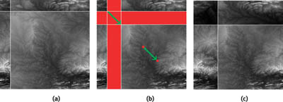
Figure 2-8 Processing a Toroidal Update
To facilitate terrain compression and synthesis, elevation data in the update region is first predicted by upsampling the coarser level, and a residual signal is then added to provide the detail. The next sections describe the three basic steps of the update process: upsampling the coarser-level elevation data, adding the residuals, and computing the normal map.
2.4.1 Upsampling
The finer-level geometry is predicted from the coarser one using an interpolatory subdivision scheme. We use the tensor-product version of the well-known four-point subdivision curve interpolant, which has mask weights ( )(Kobbelt 1996). This upsampling filter has the desirable property of being C1 smooth.
Depending on the position of the sample in the grid (even-even, even-odd, odd-even, odd-odd), a different mask is used. For an even-even pixel, only 1 texture lookup is needed because the sample is simply interpolated; for an odd-odd pixel, 4x4 texture lookups are needed; the remaining two cases require 4 texture lookups. On the CPU, the mask to be used can be easily deduced using an "if" statement. However, branch statements are expensive in the pixel shader. Hence, we always do 16 texture lookups but apply a different mask based on a lookup in a 2x2 texture.
The HLSL code for the upsampling shader appears in Listing 2-3. Code for the missing functions Upsample and ZCoarser is included on the accompanying CD.
Example 2-3. Pixel Shader Code for Creating/Updating a Clipmap Elevation Map
// residualSampler: 2D texture containing residuals, which can be
//
either decompressed data or synthesized noise
                                // p_uv: coordinates of the grid sample
                                uniform float2 Scale;
// Pixel shader for updating the elevation map
float4 UpsamplePS(float2 p_uv : TEXCOORD0) : COLOR
{
  float2 uv = floor(p_uv);
  // the Upsample() function samples the coarser elevation map
  //
using a linear interpolatory filter with 4x4 taps
// (depending on the even/odd configuration of location uv,
//
it applies 1 of 4 possible masks)
float z_predicted = Upsample(uv); // details omitted here
// add the residual to get the actual elevation
float residual = tex2D(residualSampler, p_uv * Scale);
float zf = z_predicted + residual;
// zf should always be an integer, since it gets packed
//
into the integer component of the floating - point texture zf = floor(zf);
// compute zc by linearly interpolating the vertices of the
//
coarse - grid edge on which the sample p_uv lies float zc =
    ZCoarser(uv); // details omitted here
float zd = zc - zf;
// pack the signed difference zd into the fractional component
float zf_zd = zf + (zd + 256) / 512;
return float4(zf_zd, 0, 0, 0);
}
2.4.2 Residuals
The residuals added to the upsampled coarser data can come from either decompression or synthesis.
In the compressed representation, the residual data is encoded using image compression. We use a particular lossy image coder called PTC because it supports efficient region-of-interest decoding (Malvar 2000). The CPU performs the decompression and stores the result into a residual texture image.
Alternatively, we synthesize fractal detail by letting the residuals be uncorrelated Gaussian noise (Fournier et al. 1982). This synthesis is made extremely fast on the GPU by reading a small precomputed 2D texture containing Gaussian noise. We enable texture wrapping to extend the Gaussian texture infinitely, and apply a small magnification to the texture coordinates to break the regular periodicity. The superposition of noise across the many resolution levels gives rise to a terrain without any visible repetitive patterns, as Figure 2-9 shows.
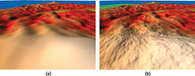
Figure 2-9 On-the-Fly Terrain Synthesis
2.4.3 Normal Map
The shader that updates the normal map for a level takes as input the elevation map at the same level. It computes the current normal as the cross product of two grid-aligned tangent vectors. Additionally, it does a texture lookup to gather the normal from the coarser level. Finally, it packs (N x , N y , N cx , N cy ) into the four-channel texture. The code is included in the accompanying CD.
2.5 Results and Discussion
Our main data set is a 216,000x93,600 height map of the conterminous United States at 30-meter spacing and 1.0-meter vertical resolution. It compresses by a factor of more than 100 and therefore fits in only 355 MB of system memory. We render this terrain into a 1024x768 window on a PC with a 2.4 GHz Pentium 4, 1 GB system memory, and an NVIDIA GeForce 6800 GT.
Rendering rate: For L = 11 levels of size n = 255, we obtain 130 frames/sec with view frustum culling, at a rendering rate of 60 million triangles/sec. The use of a vertex-texture lookup is a bottleneck, since removing the lookup increases rendering rate to 185 frames/sec. (For n = 127, the rate with vertex textures is 298 frames/sec.)
Update rate: Table 2-2 shows the processing times for the various steps of the update process, for the extreme case of updating a whole level at once. Decompression on the CPU is clearly the bottleneck of the update process.
Table 2-2. Update Times for Processing an Entire 255x255 Level
|
These are worst-case numbers because, in general, during smooth viewer motions, only small fractions of a full level need be updated per frame. |
||
|
Previous Implementation [*] |
GPU-Based Implementation |
|
|
Upsampling |
3 ms |
1.0 ms |
|
Decompression |
8 ms |
8 ms [**] |
|
Synthesis |
3 ms |
~0 ms |
|
Normal-Map Computation |
11 ms |
0.6 ms |
Final frame rate: For decompressed terrains, the system maintains a rate of around 87 frames/sec during viewer motion, and for synthesized terrains, the frame rate is about 120 frames/sec.
2.6 Summary and Improvements
We have presented a GPU implementation of the geometry clipmap framework. The representation of geometry using regular grids allows nearly all computation to proceed on the graphics card, thereby offloading work from the CPU. The system supports interactive flight over a 20-billion-sample grid of the U.S. data set stored in just 355 MB of memory at around 90 frames/sec.
2.6.1 Vertex Textures
Geometry clipmaps use vertex textures in a very special, limited way: the texels are accessed essentially in raster-scan order, and in one-to-one correspondence with vertices. Thus, we can hope for future mechanisms that would allow increased rendering efficiency.
2.6.2 Eliminating Normal Maps
It should be possible to directly compute normals in the pixel shader by accessing four filtered samples of the elevation map. At present, vertex texture lookups require that the elevation maps be stored in 32-bit floating-point images, which do not support efficient bilinear filtering.
2.6.3 Memory-Free Terrain Synthesis
Fractal terrain synthesis is so fast on the GPU that we can consider regenerating the clipmap levels during every frame, thereby saving video memory. We allocate two textures, T 1 and T 2, and toggle between them as follows. Let T 1 initially contain the coarse geometry used to seed the synthesis process. First, we use T 1 as a source texture in the update pixel shader to upsample and synthesize the next-finer level into the destination texture T 2. Second, we use T 1 as a vertex texture to render its clipmap ring. Then, we swap the roles of the two textures and iterate the process until all levels are synthesized and rendered. Initial experiments are extremely promising, with frame rates of about 59 frames/sec using L = 9 levels.
2.7 References
Fournier, Alain, Don Fussell, and Loren Carpenter. 1982. "Computer Rendering of Stochastic Models." Communications of the ACM 25(6), June 1982, pp. 371–384.
Gerasimov, Philip, Randima Fernando, and Simon Green. 2004. "Shader Model 3.0: Using Vertex Textures." NVIDIA white paper DA-01373-001_v00, June 2004. Available online at http://developer.nvidia.com/object/using_vertex_textures.html.
Kobbelt, Leif. 1996. "Interpolatory Subdivision on Open Quadrilateral Nets with Arbitrary Topology." In Eurographics 1996, pp. 409–420.
Losasso, Frank, and Hugues Hoppe. 2004. "Geometry Clipmaps: Terrain Rendering Using Nested Regular Grids." ACM Transactions on Graphics (Proceedings of SIGGRAPH 2004) 23(3), pp. 769–776.
Malvar, Henrique. 2000. "Fast Progressive Image Coding without Wavelets." In Data Compression Conference (DCC '00), pp. 243–252.
Tanner, Christopher, Christopher Migdal, and Michael Jones. 1998. "The Clipmap: A Virtual Mipmap." In Computer Graphics (Proceedings of SIGGRAPH 98), pp. 151–158.
Copyright
Many of the designations used by manufacturers and sellers to distinguish their products are claimed as trademarks. Where those designations appear in this book, and Addison-Wesley was aware of a trademark claim, the designations have been printed with initial capital letters or in all capitals.
The authors and publisher have taken care in the preparation of this book, but make no expressed or implied warranty of any kind and assume no responsibility for errors or omissions. No liability is assumed for incidental or consequential damages in connection with or arising out of the use of the information or programs contained herein.
NVIDIA makes no warranty or representation that the techniques described herein are free from any Intellectual Property claims. The reader assumes all risk of any such claims based on his or her use of these techniques.
The publisher offers excellent discounts on this book when ordered in quantity for bulk purchases or special sales, which may include electronic versions and/or custom covers and content particular to your business, training goals, marketing focus, and branding interests. For more information, please contact:
U.S. Corporate and Government Sales
(800) 382-3419
corpsales@pearsontechgroup.com
For sales outside of the U.S., please contact:
International Sales
international@pearsoned.com
Visit Addison-Wesley on the Web: www.awprofessional.com
Library of Congress Cataloging-in-Publication Data
GPU gems 2 : programming techniques for high-performance graphics and general-purpose
computation / edited by Matt Pharr ; Randima Fernando, series editor.
p. cm.
Includes bibliographical references and index.
ISBN 0-321-33559-7 (hardcover : alk. paper)
1. Computer graphics. 2. Real-time programming. I. Pharr, Matt. II. Fernando, Randima.
T385.G688 2005
006.66—dc22
2004030181
GeForce™ and NVIDIA Quadro® are trademarks or registered trademarks of NVIDIA Corporation.
Nalu, Timbury, and Clear Sailing images © 2004 NVIDIA Corporation.
mental images and mental ray are trademarks or registered trademarks of mental images, GmbH.
Copyright © 2005 by NVIDIA Corporation.
All rights reserved. No part of this publication may be reproduced, stored in a retrieval system, or transmitted, in any form, or by any means, electronic, mechanical, photocopying, recording, or otherwise, without the prior consent of the publisher. Printed in the United States of America. Published simultaneously in Canada.
For information on obtaining permission for use of material from this work, please submit a written request to:
Pearson Education, Inc.
Rights and Contracts Department
One Lake Street
Upper Saddle River, NJ 07458
Text printed in the United States on recycled paper at Quebecor World Taunton in Taunton, Massachusetts.
Second printing, April 2005
Dedication
To everyone striving to make today's best computer graphics look primitive tomorrow
- Copyright
- Inside Back Cover
- Inside Front Cover
- Part I: Geometric Complexity
-
- Chapter 1. Toward Photorealism in Virtual Botany
- Chapter 2. Terrain Rendering Using GPU-Based Geometry Clipmaps
- Chapter 3. Inside Geometry Instancing
- Chapter 4. Segment Buffering
- Chapter 5. Optimizing Resource Management with Multistreaming
- Chapter 6. Hardware Occlusion Queries Made Useful
- Chapter 7. Adaptive Tessellation of Subdivision Surfaces with Displacement Mapping
- Chapter 8. Per-Pixel Displacement Mapping with Distance Functions
- Part II: Shading, Lighting, and Shadows
-
- Chapter 9. Deferred Shading in S.T.A.L.K.E.R.
- Chapter 10. Real-Time Computation of Dynamic Irradiance Environment Maps
- Chapter 11. Approximate Bidirectional Texture Functions
- Chapter 12. Tile-Based Texture Mapping
- Chapter 13. Implementing the mental images Phenomena Renderer on the GPU
- Chapter 14. Dynamic Ambient Occlusion and Indirect Lighting
- Chapter 15. Blueprint Rendering and "Sketchy Drawings"
- Chapter 16. Accurate Atmospheric Scattering
- Chapter 17. Efficient Soft-Edged Shadows Using Pixel Shader Branching
- Chapter 18. Using Vertex Texture Displacement for Realistic Water Rendering
- Chapter 19. Generic Refraction Simulation
- Part III: High-Quality Rendering
-
- Chapter 20. Fast Third-Order Texture Filtering
- Chapter 21. High-Quality Antialiased Rasterization
- Chapter 22. Fast Prefiltered Lines
- Chapter 23. Hair Animation and Rendering in the Nalu Demo
- Chapter 24. Using Lookup Tables to Accelerate Color Transformations
- Chapter 25. GPU Image Processing in Apple's Motion
- Chapter 26. Implementing Improved Perlin Noise
- Chapter 27. Advanced High-Quality Filtering
- Chapter 28. Mipmap-Level Measurement
- Part IV: General-Purpose Computation on GPUS: A Primer
-
- Chapter 29. Streaming Architectures and Technology Trends
- Chapter 30. The GeForce 6 Series GPU Architecture
- Chapter 31. Mapping Computational Concepts to GPUs
- Chapter 32. Taking the Plunge into GPU Computing
- Chapter 33. Implementing Efficient Parallel Data Structures on GPUs
- Chapter 34. GPU Flow-Control Idioms
- Chapter 35. GPU Program Optimization
- Chapter 36. Stream Reduction Operations for GPGPU Applications
- Part V: Image-Oriented Computing
-
- Chapter 37. Octree Textures on the GPU
- Chapter 38. High-Quality Global Illumination Rendering Using Rasterization
- Chapter 39. Global Illumination Using Progressive Refinement Radiosity
- Chapter 40. Computer Vision on the GPU
- Chapter 41. Deferred Filtering: Rendering from Difficult Data Formats
- Chapter 42. Conservative Rasterization
- Part VI: Simulation and Numerical Algorithms
-
- Chapter 43. GPU Computing for Protein Structure Prediction
- Chapter 44. A GPU Framework for Solving Systems of Linear Equations
- Chapter 45. Options Pricing on the GPU
- Chapter 46. Improved GPU Sorting
- Chapter 47. Flow Simulation with Complex Boundaries
- Chapter 48. Medical Image Reconstruction with the FFT