
GPU Gems 2
GPU Gems 2 is now available, right here, online. You can purchase a beautifully printed version of this book, and others in the series, at a 30% discount courtesy of InformIT and Addison-Wesley.
The CD content, including demos and content, is available on the web and for download.
Chapter 31. Mapping Computational Concepts to GPUs
Mark Harris
NVIDIA Corporation
Recently, graphics processors have emerged as a powerful computational platform. A variety of encouraging results, mostly from researchers using GPUs to accelerate scientific computing and visualization applications, have shown that significant speedups can be achieved by applying GPUs to data-parallel computational problems. However, attaining these speedups requires knowledge of GPU programming and architecture.
The preceding chapters have described the architecture of modern GPUs and the trends that govern their performance and design. Continuing from the concepts introduced in those chapters, in this chapter we present intuitive mappings of standard computational concepts onto the special-purpose features of GPUs. After presenting the basics, we introduce a simple GPU programming framework and demonstrate the use of the framework in a short sample program.
31.1 The Importance of Data Parallelism
As with any computer, attaining maximum performance from a GPU requires some understanding of its architecture. The previous two chapters provide a good overview of GPU architecture and the trends that govern its evolution. As those chapters showed, GPUs are designed for computer graphics, which has a highly parallel style of computation that computes output streams of colored pixels from input streams of independent data elements in the form of vertices and texels. To do this, modern GPUs have many programmable processors that apply kernel computations to stream elements in parallel.
The design of GPUs is essential to keep in mind when programming them—whether for graphics or for general-purpose computation. In this chapter, we apply the stream processing concepts introduced in Chapter 29, "Streaming Architectures and Technology Trends," to general-purpose computation on GPUs (GPGPU). The biggest difficulty in applying GPUs to general computational problems is that they have a very specialized design. As a result, GPU programming is entrenched in computer graphics APIs and programming languages. Our goal is to abstract from those APIs by drawing analogies between computer graphics concepts and general computational concepts. In so doing, we hope to get you into the data-parallel frame of mind that is necessary to make the most of the parallel architecture of GPUs.
31.1.1 What Kinds of Computation Map Well to GPUs?
Before we get started, let's get an idea of what GPUs are really good at. Clearly they are good at computer graphics. Two key attributes of computer graphics computation are data parallelism and independence: not only is the same or similar computation applied to streams of many vertices and fragments, but also the computation on each element has little or no dependence on other elements.
Arithmetic Intensity
These two attributes can be combined into a single concept known as arithmetic intensity, which is the ratio of computation to bandwidth, or more formally:
|
arithmetic intensity = operations / words transferred. |
As discussed in Chapter 29, the cost of computation on microprocessors is decreasing at a faster rate than the cost of communication. This is especially true of parallel processors such as GPUs, because as technology improvements make more transistors available, more of these transistors are applied to functional units (such as arithmetic logic units) that increase computational throughput, than are applied to memory hierarchy (caches) that decrease memory latency. Therefore, GPUs demand high arithmetic intensity for peak performance.
As such, the computations that benefit most from GPU processing have high arithmetic intensity. A good example of this is the solution of systems of linear equations. Chapter 44, "A GPU Framework for Solving Systems of Linear Equations," discusses the efficient representation of vectors and matrices and how to use this representation to rapidly solve linear partial differential equations. These computations perform well on GPUs because they are highly data-parallel: they consist of large streams of data elements (in the form of matrices and vectors), to which identical computational kernels are applied. The data communication required to compute each element of the output is small and coherent. As a result, the number of data words transferred from main memory is kept low and the arithmetic intensity is high.
Other examples of computation that works well on GPUs include physically based simulation on lattices, as discussed in Chapter 47, "Flow Simulation with Complex Boundaries," and all-pairs shortest-path algorithms, as described in Chapter 43, "GPU Computing for Protein Structure Prediction."
31.1.2 Example: Simulation on a Grid
For the rest of this chapter, we employ a simple but effective example: simulating natural phenomena on a grid. The Cartesian grid shown in Figure 31-1 is a discrete representation of the 2D spatial domain on which our phenomenon evolves. The example in this case is a physically based cloud simulation. We won't go into the physical and mathematical detail of this simulation, except to illustrate some basic GPGPU concepts. For more information on cloud simulation, see Harris et al. 2003.

Figure 31-1 Simulation on a Grid
Computation on a grid is common in GPGPU, because grids have a natural representation on GPUs: textures. Also, GPUs contain small texture caches that are optimized for 2D data locality, unlike the 1D data caches employed in CPUs. Many computations map naturally to grids, including matrix algebra; image and volume processing; physically based simulation; and global illumination algorithms such as ray tracing, photon mapping, and radiosity (see Chapter 39, "Global Illumination Using Progressive Refinement Radiosity"). Computations that aren't naturally performed on grids can also be mapped to grid computation by converting 1D addresses into 2D addresses.
The cloud simulation algorithm consists of a number of steps, as shown in Figure 31-1. The important detail about the algorithm steps is that each step updates the entire grid, and each step must complete before the next proceeds. In stream processing terms, the data stored in the grid cells make up our streams, and the algorithm steps are our computational kernels. Each kernel is applied to each stream element, generating a new stream that becomes the input to the next step.
31.1.3 Stream Communication: Gather vs. Scatter
High arithmetic intensity requires that communication between stream elements be minimized, but for many computations, communication is a necessary evil. In the cloud simulation, for example, some of the kernels must obtain information from cells other than the one currently being processed by the kernel. When discussing data communication on GPUs, it is helpful to consider two main types of communication: gather and scatter. Gather occurs when the kernel processing a stream element requests information from other elements in the stream: it "gathers" information from other parts of memory. Scatter, on the other hand, occurs when the kernel processing a stream element distributes information to other stream elements: it "scatters" information to other parts of memory. In terms of traditional memory concepts, gather requires only random-access load capability, while scatter requires only random-access store capability. Later we show why gather is typically preferable to scatter.
31.2 An Inventory of GPU Computational Resources
To start mapping general computation onto the specialized hardware of a GPU, we should first survey the computational resources that GPUs provide. We start with the computational workhorses: the processors.
31.2.1 Programmable Parallel Processors
GPUs have two types of programmable processors: vertex processors and fragment processors. Vertex processors process streams of vertices (made up of positions, colors, normal vectors, and other attributes), which are the elements that compose polygonal geometric models. Computer graphics typically represents 3D objects with triangular meshes. The vertex processors apply a vertex program(sometimes called a vertex shader) to transform each vertex based on its position relative to the camera, and then each set of three vertices is used to compute a triangle, from which streams of fragments are generated. A fragment can be considered a "proto-pixel." It contains all information needed to generate a shaded pixel in the final image, including color, depth, and destination in the frame buffer. The fragment processors apply a fragment program (sometimes called a pixel shader) to each fragment in the stream to compute the final color of each pixel.
Vertex Processors
Modern GPUs have multiple vertex processors (the NVIDIA GeForce 6800 Ultra and the ATI Radeon X800 XT both have six). These processors are fully programmable and operate in either SIMD- or MIMD-parallel fashion on the input vertices (see Chapter 34 for more information on these terms). The basic primitives of 3D computer graphics are 3D vertices in projected space, represented by an (x, y, z, w) vector, and four-component colors stored as (red, green, blue, alpha) vectors (often abbreviated RGBA), where alpha typically represents an opacity percentage. Because of this, vertex processors have hardware to process four-component vectors. This allows them to produce transformed vertex positions in fewer cycles.
Vertex processors are capable of changing the position of input vertices. If you think about this, the position of these vertices ultimately affects where in the image pixels will be drawn. An image is nothing but an array of memory; thus, because vertex processors can control where in memory data will be written, they are thus capable of scatter. However, most current vertex processors cannot directly read information from vertex elements in the input stream other than the one currently being processed. Therefore, they are incapable of gather. The NVIDIA GeForce 6 Series GPUs have a new feature called vertex texture fetch (VTF). This means that GeForce 6 vertex processors are capable of random-access memory reads. So, we can store part or all of our input stream data in a vertex texture and use VTF to implement a gather operation.
Fragment Processors
Modern GPUs also have multiple fragment processors (the NVIDIA GeForce 6800 Ultra and the ATI X800 XT both have 16). Like vertex processors, these are fully programmable. Fragment processors operate in SIMD-parallel fashion on input elements, processing four-element vectors in parallel. Fragment processors have the ability to fetch data from textures, so they are capable of gather. However, the output address of a fragment is always determined before the fragment is processed: the processor cannot change the output location of a pixel. Fragment processors are thus not natively capable of scatter. However, see Section 31.3 for further discussion and techniques for working around this limitation.
For GPGPU applications, the fragment processors are typically used more heavily than the vertex processors. There are two main reasons for this. First, there are more fragment processors than vertex processors on a typical programmable GPU. Second, the output of the fragment processors goes more or less directly into memory, which can be fed straight back in as a new stream of texture data. Vertex processor output, on the other hand, must pass through the rasterizer and fragment processors before reaching memory. This makes direct output from vertex processors less straightforward.
Rasterizer
As mentioned earlier, after the vertex processors transform vertices, each group of three vertices is used to compute a triangle (in the form of edge equations), and from this triangle a stream of fragments is generated. This work of generating fragments is done by the rasterizer. We can think of the rasterizer as an address interpolator. Later we show how memory addresses are represented as texture coordinates. The rasterizer interpolates these addresses and other per-vertex values based on the fragment position. Because it generates many data elements from only a few input elements, we can also think of the rasterizer as a data amplifier. These functions of the rasterizer are very specialized to rendering triangles and are not user-programmable.
Texture Unit
Fragment processors (and vertex processors on the latest GPUs) can access memory in the form of textures. We can think of the texture unit as a read-only memory interface.
Render-to-Texture
When an image is generated by the GPU, it can be written to frame-buffer memory that can be displayed, or it can be written to texture memory. This render-to-texture functionality is essential for GPGPU, because it is the only current mechanism with which to implement direct feedback of GPU output to input without going back to the host processor. (Indirect feedback is also available via copy-to-texture, which requires a copy from one location in the GPU's memory to another.) We can think of render-to-texture as a write-only memory interface.
You may be wondering why we don't consider the texture unit and render-to-texture together as a read-write memory interface. The reason is that the fragment processor can read memory as many times as it wants inside a kernel, but it can write data only at the end of the kernel program (this is stream out). Thus, memory reads and writes are fundamentally separate on GPUs, so it helps to think about them that way.
Data Types
When programming CPUs, we are used to dealing with multiple data types, such as integers, floats, and Booleans. Current GPUs are more limited in this regard. Although some of the high-level shading languages used by GPUs expose integer and Boolean data types, current GPUs process only real numbers in the form of fixed- or floating-point values. Also, there are multiple floating-point formats supported by current GPUs. For example, NVIDIA GeForce FX and GeForce 6 Series GPUs support both 16-bit (a sign bit, 10 mantissa bits, and 5 exponent bits) and 32-bit (a sign bit, 23 mantissa bits, and 8 exponent bits: identical to the IEEE-754 standard) floating-point formats. All current ATI products, including the Radeon 9800 and X800, support a 24-bit floating-point format, with a sign bit, 16 mantissa bits, and 7 exponent bits. The lack of integer data types on GPUs is a current limitation. This can typically be worked around using floating-point numbers, but, for example, not all 32-bit integers can be represented in 32-bit floating-point format (because there are only 23 bits in the mantissa). One must be careful because floating-point numbers cannot exactly represent the same range of whole numbers that their same-size integer counterparts can represent. Table 31-1 shows the bit fields of each floating-point format and a description of the values they can represent.
Table 31-1. Floating-Point Formats Currently Supported by NVIDIA and ATI GPUs
|
Name |
Sign |
Exponent |
Mantissa |
Largest Values |
Smallest Values |
Whole Number Range [1] |
Supports Specials (NaN, Inf, etc.) |
|
NVIDIA 16-bit |
15 (1) |
14:10 (5) |
9:0 (10) |
±65,504 |
±2- 14 |
±2048 |
Yes |
|
ATI 16-bit |
15 (1) |
14:10 (5) |
9:0 (10) |
±131,008 |
±2- 15 |
±2048 |
No |
|
ATI 24-bit |
23 (1) |
22:16 (7) |
15:0 (16) |
±~264 |
±~2- 62 |
±131,072 |
No |
|
NVIDIA 32-bit (IEEE 754) |
31 (1) |
30:23 (8) |
22:0 (23) |
±~2128 |
±~2- 126 |
±16,777,216 |
Yes |
 10- 5 (±2- 24 with denorms)
31.3 CPU-GPU Analogies
Even for expert CPU programmers, getting started in GPU programming can be tricky without some knowledge of graphics programming. In this section, we try to aid your understanding by drawing some very simple analogies between traditional CPU computational concepts and their GPU counterparts. We start with the concept of streams and kernels.
31.3.1 Streams: GPU Textures = CPU Arrays
This one is easy. The fundamental array data structures on GPUs are textures and vertex arrays. As we observed before, fragment processors tend to be more useful for GPGPU than vertex processors. Therefore, anywhere we would use an array of data on the CPU, we can use a texture on the GPU.
31.3.2 Kernels: GPU Fragment Programs = CPU "Inner Loops"
The many parallel processors of a GPU are its computational workhorses—they perform the kernel computation on data streams. On the CPU, we would use a loop to iterate over the elements of a stream (stored in an array), processing them sequentially. In the CPU case, the instructions inside the loop are the kernel. On the GPU, we write similar instructions inside a fragment program, which are applied to all elements of the stream. The amount of parallelism in this computation depends on the number of processors on the GPU we use, but also on how well we exploit the instruction-level parallelism enabled by the four-vector structure of GPU arithmetic. Note that vertex programs can also be thought of as kernels operating on a stream of vertices.
31.3.3 Render-to-Texture = Feedback
As mentioned before, most computations are broken into steps. Each step depends on the output of previous steps. In terms of streams, typically a kernel must process an entire stream before the next kernel can proceed, due to dependencies between stream elements. Also, in the case of physically based simulation, each time step of the simulation depends on the results of the previous time step.
All of this feedback is trivial to implement on the CPU because of its unified memory model, in which memory can be read or written anywhere in a program. Things aren't so easy on the GPU, as we discussed before. To achieve feedback, we must use render-to-texture to write the results of a fragment program to memory so they can then be used as input to future programs.
31.3.4 Geometry Rasterization = Computation Invocation
Now we have analogies for data representation, computation, and feedback. To run a program, though, we need to know how to invoke computation. Our kernels are fragment programs, so all we need to know is how to generate streams of fragments. This should be clear from the previous section; to invoke computation, we just draw geometry. The vertex processors will transform the geometry, and the rasterizer will determine which pixels in the output buffer it covers and generate a fragment for each one.
In GPGPU, we are typically processing every element of a rectangular stream of fragments representing a grid. Therefore, the most common invocation in GPGPU programming is a single quadrilateral.
31.3.5 Texture Coordinates = Computational Domain
Each kernel (fragment program) that executes on the GPU takes a number of streams as input and typically generates one stream of output. Newer GPUs that support multiple render targets can generate multiple output streams (currently limited to four RGBA streams). Any computation has an input domain and an output range. In many cases, the domain of a computation on the GPU may have different dimensions than the input streams.
GPUs provide a simple way to deal with this, in the form of texture coordinates. These coordinates are stored at vertices, and the rasterizer linearly interpolates the coordinates at each vertex to generate a set of coordinates for each fragment. The interpolated coordinates are passed as input to the fragment processor. In computer graphics, these coordinates are used as indices for texture fetches. For GPGPU, we can think of them as array indices, and we can use them to control the domain of the computation. The domain and range may be the same size, or the domain can be smaller than the range (data amplification/magnification), or the domain can be larger than the range (data minification). The rasterizer makes it easy to correctly sample the input stream at the correct intervals for each of these cases.
31.3.6 Vertex Coordinates = Computational Range
As discussed before, fragments are generated from input geometry by the rasterizer, and these fragments become output pixels after fragment processing. Because the fragment processors are not directly capable of scatter, the input vertices and the vertex program determine which pixels are generated. Typically, we specify four vertices of a quad in output pixel coordinates and apply a vertex program that simply passes the vertices through untransformed. Thus, vertex coordinates directly control the output range of the computation.
31.3.7 Reductions
Everything we've discussed up to this point has assumed purely parallel computation: each element is computed largely independently of the rest of the stream. However, there are times when we need to reduce a large vector of values to a smaller vector, or even to a single value. For example, we might need to compute the sum or the maximum of all values in an array. This sort of computation is called a parallel reduction.
On GPUs, reductions can be performed by alternately rendering to and reading from a pair of buffers. On each pass, the size of the output (the computational range) is reduced by some fraction. To produce each element of the output, a fragment program reads two or more values and computes a new one using the reduction operator, such as addition or maximum. These passes continue until the output is a single-element buffer, at which point we have our reduced result. In general, this process takes O(log n) passes, where n is the number of elements to reduce. For example, for a 2D reduction, the fragment program might read four elements from four quadrants of the input buffer, such that the output size is halved in both dimensions at each step. Figure 31-2 demonstrates a max reduction on a 2D buffer.
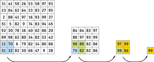
Figure 31-2 Max Reduction Performed with Multiple Passes
31.4 From Analogies to Implementation
By now you have a high-level understanding of how most GPGPU programs operate on current GPUs. The analogies from the previous section provide us a general implementation plan. Now, so that you can start putting the GPU to work, we dig into the nitty-gritty implementation details that you will need in practice.
31.4.1 Putting It All Together: A Basic GPGPU Framework
To make this easy, we've put together a very basic framework in C++ that you can use to write GPGPU programs. You'll find the framework on the CD included with this book. The framework, called pug, incorporates all of the analogies from the previous section in order to abstract GPGPU programming in a manner more accessible to experienced CPU programmers.
Initializing and Finalizing a GPGPU Application
The first step in a GPGPU application is to initialize the GPU. This is very easy in the framework: just call pugInit(). When the application is finished with the GPU, it can clean up the memory used by the graphics API by calling pugCleanup().
Specifying Kernels
Kernels in our framework are written in the Cg language. Although Cg is designed for graphics, it is based on the C language and therefore is very easy to learn. For more information, we recommend The Cg Tutorial (Fernando and Kilgard 2003) and the documentation included with the Cg distribution (NVIDIA 2004). There are very few graphics-specific keywords in Cg. We provide a Cg file, pug.cg, that you can include in your kernel files. This file defines a structure called Stream that abstracts the most graphics-centric concept: texture fetching. Stream is a wrapper for the texture sampler Cg type. Calling one of the value() functions of the Stream structure gives the value of a stream element.
To load and initialize a kernel program from a file, use the pugLoadProgram() function. The function returns a pointer to a PUGProgram structure, which you will need to store and pass to the other framework functions to bind constants and streams to the kernel and to run it.
Stream Management
Arrays of data in the framework are called buffers. The pugAllocateBuffer() function creates a new buffer. Buffers can be read-only, write-only, or read-write, and this can be specified using the mode parameter of this function. This function returns a pointer to a PUGBuffer structure, which can be passed to a number of functions in the framework, including the following two.
To load initial data into a buffer, pass the data to the pugInitBuffer() function.
To bind an input stream for a kernel to a buffer, call pugBindStream(), which takes as arguments a pointer to the PUGProgram to bind to, the PUGBuffer pointer, and a string containing the name of the Stream parameter in the Cg kernel program to which this PUGBuffer should be bound.
Specifying Computational Domain and Range
To specify the domain and range of a computation, define a PUGRect structure with the coordinates of the corners of the rectangle that should be used as either the domain or range. Multiple domains can be specified. These will generate additional texture coordinates that the kernel program can use as needed.
To bind a domain, call pugBindDomain(), passing it the PUGProgram, a string parameter name for this domain defined in the kernel Cg program, and the PUGRect for the domain.
There can be only one range for a kernel, due to the inability of fragment programs to scatter. To specify the range, simply pass a PUGRect to the range parameter of the pugRunProgram() function.
Specifying Constant Parameters
Constant one-, two-, three-, or four-component floating-point parameters can be specified using pugBindFloat(), which takes as arguments a pointer to the PUGProgram, a string parameter name, and up to four floating-point values.
Invoking a Kernel
Once the preceding steps have been done, executing the computation is simple: just call the function pugRunProgram(). Pass it a pointer to the PUGProgram, the output PUGBuffer (which must be writable), and an optional PUGRect to specify the range. The entire buffer will be written if the range is not specified.
Note that a stream cannot be bound to a buffer if that buffer is currently being used for the output of a kernel. The framework will automatically release all streams bound to any buffer that is specified as the output buffer in pugRunProgram().
Getting Data Back to the CPU
To bring results on the GPU back to the CPU, call the pugGetBufferData() function, passing it a pointer to the PUGBuffer. This function returns a pointer to a C array of type float. Reading data back from the GPU can cause the GPU pipeline to flush, so use this function sparingly to avoid hurting application performance.
Parallel Reductions
The framework provides support for three types of simple parallel reduction. Buffers can be reduced along rows (to a single column vector), along columns (to a single row vector), or both (to a single value). The framework functions for these operations are pugReduce1D() and pugReduce2D().
31.5 A Simple Example
As a basic but nontrivial GPGPU example, we use a simulation of a phenomenon known as chemical reaction-diffusion. Reaction-diffusion is a model of how the concentrations of two or more reactants in a solution evolve in space and time as they undergo the processes of chemical reaction and diffusion. The reaction-diffusion model we use is called the Grey-Scott model (Pearson 1993) and involves just two chemical reactants. This phenomenological model does not represent a particular real chemical reaction; it serves as a simple model for studying the general reaction-diffusion phenomenon. Figure 31-3 shows the results of many iterations of the Grey-Scott model.
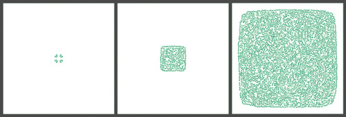
Figure 31-3 Visualizing the Grey-Scott Model
Grey-Scott consists of two simple partial differential equations that govern the evolution of the concentrations of two chemical reactants, U and V:
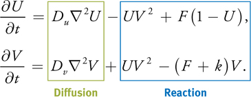
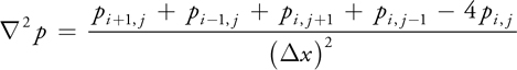
Here k and F are constants; Du and Dv are the diffusion rates of the reactants; and  2 is the Laplacian operator, which represents diffusion. The Laplacian operator appears commonly in physics, most notably in the form of diffusion equations, such as the heat equation. A finite difference form of the Laplacian operator applied to a scalar field p on a two-dimensional Cartesian grid (with indices i, j, and cell size x) is
The implementation of the Grey-Scott model is fairly simple. There is a single data stream: the U and V chemical concentrations are stored in two channels of a single texture that represents a discrete spatial grid. This stream serves as input to a simple kernel, which implements the preceding equations in discrete form. The kernel is shown in Listing 31-1. C code that uses the framework to implement the simulation is shown in Listing 31-2.
Example 31-1. The Reaction-Diffusion Kernel Program
float4 rd(float2 coords
          : DOMAIN, uniform stream concentration, uniform float2 DuDv,
            uniform float F, uniform float k)
    : RANGE
{
  float2 center = concentration.value2(coords).xy;
  float2 diffusion = concentration.value2(coords + half2(1, 0));
  diffusion += concentration.value2(coords + half2(-1, 0));
  diffusion += concentration.value2(coords + half2(0, 1));
  diffusion += concentration.value2(coords + half2(0, -1));
  // Average and scale by diffusion coeffs
  diffusion *= 0.25f * DuDv;
  float2 reaction = center.xx * center.yy * center.yy;
  reaction.x = -1;
  reaction.x += (1 - DuDv.x) * center.x + F * (1 - center.x);
  reaction.y += (-F - k + (1 - DuDv.y)) * center.y;
  // Now add the diffusion to the reaction to get the result.
  return float4(diffusion + reaction, 0, 0);
}
Example 31-2. C++ Code to Set Up and Run a Reaction-Diffusion Simulation on the GPU
See the source code on the accompanying CD for more details.
PUGBuffer *rdBuffer;
PUGProgram *rdProgram;
void init_rd()
{ // Call this once.
  pugInit();
  // Start up the GPU framework
  // Create a "double-buffered" PUGBuffer. Two buffers allow the
  // simulation to alternate using one as input, one as output
  PUGBuffer *rdBuffer =
      pugAllocateBuffer(width, height, PUG_READWRITE, 4, true);
  PUGProgram *rdProgram = pugLoadProgram("rd.cg", "rd");
  pugBindFloat(rdProgram, "DuDv", du, dv); // bind parameters
  pugBindFloat(rdProgram, "F", F);
  pugBindFloat(rdProgram, "k", k);
  // Initialize the state of the simulation with values in array
  pugInitBuffer(rdBuffer, array);
}
void update_rd()
{ // Call this every iteration
  pugBindStream(rdProgram, "concentration", rdBuffer, currentSource);
  PUGRect range(0, width, 0, height);
  pugRunProgram(rdProgram, rdBuffer, range, currentTarget);
  std::swap(currentSource, currentTarget);
}
31.6 Conclusion
You should now have a good understanding of how to map general-purpose computations onto GPUs. With this basic knowledge, you can begin writing your own GPGPU applications and learn more advanced concepts. The simple GPU framework introduced in the previous section is included on this book's CD. We hope that it provides a useful starting point for your own programs.
31.7 References
Fernando, Randima, and Mark J. Kilgard. 2003. The Cg Tutorial: The Definitive Guide to Programmable Real-Time Graphics. Addison-Wesley.
Harris, Mark J., William V. Baxter III, Thorsten Scheuermann, and Anselmo Lastra. 2003. "Simulation of Cloud Dynamics on Graphics Hardware." In Proceedings of the SIGGRAPH/Eurographics Workshop on Graphics Hardware 2003, pp. 92–101.
NVIDIA Corporation. 2004. The Cg Toolkit. Available online at http://developer.nvidia.com/object/cg_toolkit.html
Pearson, John E. 1993. "Complex Patterns in a Simple System." Science 261, p. 189.
Copyright
Many of the designations used by manufacturers and sellers to distinguish their products are claimed as trademarks. Where those designations appear in this book, and Addison-Wesley was aware of a trademark claim, the designations have been printed with initial capital letters or in all capitals.
The authors and publisher have taken care in the preparation of this book, but make no expressed or implied warranty of any kind and assume no responsibility for errors or omissions. No liability is assumed for incidental or consequential damages in connection with or arising out of the use of the information or programs contained herein.
NVIDIA makes no warranty or representation that the techniques described herein are free from any Intellectual Property claims. The reader assumes all risk of any such claims based on his or her use of these techniques.
The publisher offers excellent discounts on this book when ordered in quantity for bulk purchases or special sales, which may include electronic versions and/or custom covers and content particular to your business, training goals, marketing focus, and branding interests. For more information, please contact:
U.S. Corporate and Government Sales
(800) 382-3419
corpsales@pearsontechgroup.com
For sales outside of the U.S., please contact:
International Sales
international@pearsoned.com
Visit Addison-Wesley on the Web: www.awprofessional.com
Library of Congress Cataloging-in-Publication Data
GPU gems 2 : programming techniques for high-performance graphics and general-purpose
computation / edited by Matt Pharr ; Randima Fernando, series editor.
p. cm.
Includes bibliographical references and index.
ISBN 0-321-33559-7 (hardcover : alk. paper)
1. Computer graphics. 2. Real-time programming. I. Pharr, Matt. II. Fernando, Randima.
T385.G688 2005
006.66—dc22
2004030181
GeForce™ and NVIDIA Quadro® are trademarks or registered trademarks of NVIDIA Corporation.
Nalu, Timbury, and Clear Sailing images © 2004 NVIDIA Corporation.
mental images and mental ray are trademarks or registered trademarks of mental images, GmbH.
Copyright © 2005 by NVIDIA Corporation.
All rights reserved. No part of this publication may be reproduced, stored in a retrieval system, or transmitted, in any form, or by any means, electronic, mechanical, photocopying, recording, or otherwise, without the prior consent of the publisher. Printed in the United States of America. Published simultaneously in Canada.
For information on obtaining permission for use of material from this work, please submit a written request to:
Pearson Education, Inc.
Rights and Contracts Department
One Lake Street
Upper Saddle River, NJ 07458
Text printed in the United States on recycled paper at Quebecor World Taunton in Taunton, Massachusetts.
Second printing, April 2005
Dedication
To everyone striving to make today's best computer graphics look primitive tomorrow
- Copyright
- Inside Back Cover
- Inside Front Cover
- Part I: Geometric Complexity
-
- Chapter 1. Toward Photorealism in Virtual Botany
- Chapter 2. Terrain Rendering Using GPU-Based Geometry Clipmaps
- Chapter 3. Inside Geometry Instancing
- Chapter 4. Segment Buffering
- Chapter 5. Optimizing Resource Management with Multistreaming
- Chapter 6. Hardware Occlusion Queries Made Useful
- Chapter 7. Adaptive Tessellation of Subdivision Surfaces with Displacement Mapping
- Chapter 8. Per-Pixel Displacement Mapping with Distance Functions
- Part II: Shading, Lighting, and Shadows
-
- Chapter 9. Deferred Shading in S.T.A.L.K.E.R.
- Chapter 10. Real-Time Computation of Dynamic Irradiance Environment Maps
- Chapter 11. Approximate Bidirectional Texture Functions
- Chapter 12. Tile-Based Texture Mapping
- Chapter 13. Implementing the mental images Phenomena Renderer on the GPU
- Chapter 14. Dynamic Ambient Occlusion and Indirect Lighting
- Chapter 15. Blueprint Rendering and "Sketchy Drawings"
- Chapter 16. Accurate Atmospheric Scattering
- Chapter 17. Efficient Soft-Edged Shadows Using Pixel Shader Branching
- Chapter 18. Using Vertex Texture Displacement for Realistic Water Rendering
- Chapter 19. Generic Refraction Simulation
- Part III: High-Quality Rendering
-
- Chapter 20. Fast Third-Order Texture Filtering
- Chapter 21. High-Quality Antialiased Rasterization
- Chapter 22. Fast Prefiltered Lines
- Chapter 23. Hair Animation and Rendering in the Nalu Demo
- Chapter 24. Using Lookup Tables to Accelerate Color Transformations
- Chapter 25. GPU Image Processing in Apple's Motion
- Chapter 26. Implementing Improved Perlin Noise
- Chapter 27. Advanced High-Quality Filtering
- Chapter 28. Mipmap-Level Measurement
- Part IV: General-Purpose Computation on GPUS: A Primer
-
- Chapter 29. Streaming Architectures and Technology Trends
- Chapter 30. The GeForce 6 Series GPU Architecture
- Chapter 31. Mapping Computational Concepts to GPUs
- Chapter 32. Taking the Plunge into GPU Computing
- Chapter 33. Implementing Efficient Parallel Data Structures on GPUs
- Chapter 34. GPU Flow-Control Idioms
- Chapter 35. GPU Program Optimization
- Chapter 36. Stream Reduction Operations for GPGPU Applications
- Part V: Image-Oriented Computing
-
- Chapter 37. Octree Textures on the GPU
- Chapter 38. High-Quality Global Illumination Rendering Using Rasterization
- Chapter 39. Global Illumination Using Progressive Refinement Radiosity
- Chapter 40. Computer Vision on the GPU
- Chapter 41. Deferred Filtering: Rendering from Difficult Data Formats
- Chapter 42. Conservative Rasterization
- Part VI: Simulation and Numerical Algorithms
-
- Chapter 43. GPU Computing for Protein Structure Prediction
- Chapter 44. A GPU Framework for Solving Systems of Linear Equations
- Chapter 45. Options Pricing on the GPU
- Chapter 46. Improved GPU Sorting
- Chapter 47. Flow Simulation with Complex Boundaries
- Chapter 48. Medical Image Reconstruction with the FFT