
GPU Gems 2
GPU Gems 2 is now available, right here, online. You can purchase a beautifully printed version of this book, and others in the series, at a 30% discount courtesy of InformIT and Addison-Wesley.
The CD content, including demos and content, is available on the web and for download.
Chapter 15. Blueprint Rendering and "Sketchy Drawings"
Marc Nienhaus
University of Potsdam, Hasso-Plattner-Institute
Jürgen Döllner
University of Potsdam, Hasso-Plattner-Institute
In this chapter, we present two techniques for hardware-accelerated, image-space non-photorealistic rendering: blueprint rendering and sketchy drawing.
Outlining and enhancing visible and occluded features in drafts of architecture and technical parts are essential techniques for visualizing complex aggregate objects and for illustrating the position, layout, and relation of their components. Blueprint rendering is a novel multipass rendering technique that outlines visible and nonvisible visually important edges of 3D objects. The word blueprint in its original sense is defined by Merriam-Webster as "a photographic print in white on a bright blue ground or blue on a white ground used especially for copying maps, mechanical drawings, and architects' plans." Blueprints consist of transparently rendered features, represented by their outlines. Thus, blueprints make it easy to understand the structure of complex, hierarchical object assemblies such as those found in architectural drafts, technical illustrations, and designs.
In this sense, blueprint rendering can become an effective tool for interactively exploring, visualizing, and communicating spatial relations. For instance, they can help guide players through dungeon-like environments and highlight hidden chambers and components in a computer game, or they can make it easier for artists to visualize and design game levels in a custom level editor.
In contrast, rendering in a "sketchy" manner can be used to communicate visual ideas and to illustrate drafts and concepts, especially in application areas such as architectural and product designs. In particular, sketchy drawings encourage the exchange of ideas when people are reconsidering drafts.
Sketchy drawing is a real-time rendering technique for sketching visually important edges as well as inner color patches of arbitrary 3D geometries even beyond their geometrical boundary. Generally speaking, with sketchy drawing we sketch the outline of 3D geometries to imply vagueness and "crayon in" inner color patches exceeding the sketchy outline as though they have been painted roughly. Combining both produces sketchy, cartoon-like depictions that can be applied to enhance the visual attraction of characters and 3D scenery.
Because of the way they're implemented (with depth sprite rendering) and the fact that they work on a per-object basis, both blueprint and sketchy rendering can easily be integrated into any real-time graphics application.
15.1 Basic Principles
Blueprint and sketchy renderings are both built on three basic principles: (1) to preserve images of intermediate renderings of the scene's geometry, (2) to implement an edge enhancement technique, and (3) to apply depth sprite rendering. We briefly describe these concepts in the following sections.
15.1.1 Intermediate Rendering Results
We denote 2D data derived from 3D geometry and rendered into textures as intermediate rendering results. In doing so, we implement G-buffers (Saito and Takahashi 1990) that store geometric properties of 3D geometry. (See also Chapter 9 of this book, "Deferred Shading in S.T.A.L.K.E.R.," for application of this idea to realistic rendering.) In particular, we generate a normal buffer and a z-buffer by rendering encoded normal and z-values of 3D geometry directly into 2D textures, as shown in Figure 15-1. In a multipass rendering technique, we generate intermediate rendering results once and can reuse them in subsequent rendering passes. Technically, we use render-to-texture capabilities of graphics hardware. Doing so also allows us to render high-precision (color) values to high-precision buffers (such as textures).
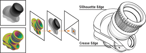
Figure 15-1 Steps in Creating an Edge Map
15.1.2 Edge Enhancement
To extract visually important edges from 3D geometry on a per-object basis, we implement an image-space edge enhancement technique (Nienhaus and Döllner 2003). Visually important edges include silhouette, border, and crease edges. We obtain these edges by detecting discontinuities in the normal buffer and z-buffer. For that purpose, we texture a screen-aligned quad that fills in the viewport of the canvas using these textures and calculate texture coordinates (s, t) for each fragment produced for the quad in such a way that they correspond to window coordinates. Sampling neighboring texels allows us to extract discontinuities that result in intensity values. The assembly of intensity values constitutes edges that we render directly into a single texture, called an edge map. Figure 15-2 depicts the normal and z-buffer and the resulting edge map.
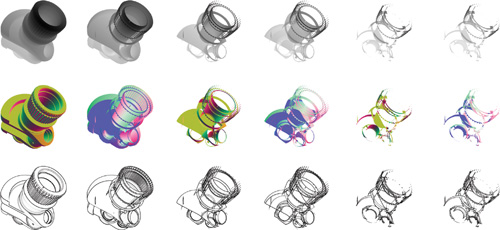
Figure 15-2 The Z-Buffer, Normal Buffer, and Edge Map for Each Layer
15.1.3 Depth Sprite Rendering
Conceptually, depth sprites are 2D images that provide an additional z-value at each pixel for depth testing. For our purposes, we implement depth sprite rendering as follows:
- We render a screen-aligned quad textured with a high-precision texture containing z-values.
- We apply a specialized fragment shader that replaces fragment z-values of the quad (produced by the rasterizer) with z-values derived from accessing the texture. For optimizing fill rate, we additionally discard a fragment if its z-value equals 1—which denotes the depth of the far clipping plane. Otherwise, the fragment shader calculates RGBA color values of that fragment.
- Rendering then proceeds with the ordinary depth test. If fragments pass the test, the frame buffer will be filled with the color and z-values of the depth sprite.
As an example in 3D scenes, depth sprite rendering can correctly resolve the visibility of image-based renderings derived from 3D geometries by considering their z-values. In particular, we can combine blueprints and sketchy drawings with other 3D geometric models in arbitrary order.
15.2 Blueprint Rendering
For blueprint rendering, we extract both visible and nonvisible edges of 3D geometry. Visible edges are edges directly seen by the virtual camera; nonvisible edges are edges that are occluded by faces of 3D geometry; that is, they are not directly seen. To extract these edges, we combine the depth-peeling technique (Everitt 2001) and the edge enhancement technique. Once generated, we compose visible and nonvisible edges as blueprints in the frame buffer.
15.2.1 Depth Peeling
Depth peeling is a technique that operates on a per-fragment basis and extracts 2D layers of 3D geometry in depth-sorted order. Generally speaking, depth peeling successively "peels away" layers of unique depth complexity.
In general, fragments passing an ordinary depth test define the minimal z-value at each pixel. But we cannot determine the fragment that comes second (or third, and so on) with respect to its depth complexity. Thus, we need an additional depth test to extract those fragments that form a layer of a given ordinal number (with respect to depth complexity) (Diefenbach 1996). We thus can extract the first n layers using n rendering passes.
We refer to a layer of unique depth complexity as a depth layer and a high-precision texture received from capturing the associated z-buffer contents as a depth layer map. Accordingly, we call the contents of the associated color buffer captured in an additional texture a color layer map. In particular, color layer maps can later be used in depth-sorted order to compose the final rendering, for example, for order-independent transparency (Everitt 2001).
The pseudocode in Listing 15-1 outlines our implementation of depth peeling. It operates on a set G of 3D geometries. We render G multiple times, whereby the rasterizer produces a set F of fragments. The loop terminates if no fragment gets rendered (termination condition); otherwise, we continue with the next depth layer. That is, if the number of rendering passes has reached the maximum depth complexity, the condition is satisfied.
Example 15-1. Pseudocode for Combining Depth Peeling and Edge Enhancement for Blueprint Rendering
 procedure depthPeeling(G
3DGeometry) begin
i=0
do
F
rasterize(G)
/* Perform single depth test in the first rendering pass */
if(i==0)
begin
for all fragment ∈ F
begin
bool test
performDepthTest(fragment)
if(test)
begin
fragment.depth
z-buffer
fragment.color
color buffer
end
else reject fragment
end
end
else begin
/* Perform two depth test */
for all fragment ∈ F
begin
if(fragment.depth > fragment.valuedepthLayerMap(i-1))
begin
/* First test */
bool test
performDepthTest(fragment)
if(test)
begin
/* Second test */
fragment.depth
z-buffer
fragment.color
color buffer
end
else reject fragment
end
else reject fragment
end
end
depthLayerMap(i)
capture(z-buffer)
colorLayerMap(i)
capture(color buffer)
/* Edge intensities */
edgeMap(i)
edges(depthLayerMap(i),colorLayerMap(i))
i++
while(occlusionQuery()
0 )
/* Termination condition */
end
Performing Two Depth Tests
In the first rendering pass (i = 0), we perform an ordinary depth test on each fragment. We capture the contents of the z-buffer and the color buffer in a depth layer map and a color layer map for further processing.
In consecutive rendering passes (i > 0), we perform an additional depth test on each fragment. For this test, we use a texture with the depth layer map of the previous rendering pass (i - 1). We then determine the texture coordinates of a fragment in such a way that they correspond to canvas coordinates of the targeted pixel position. In this way, a texture access can provide a fragment with the z-value stored at that pixel position in the z-buffer of the previous rendering pass.
Now, the two depth tests work as follows:
- If the current z-value of a fragment is greater than the texture value that results from accessing the depth layer map, the fragment proceeds and the second ordinary depth test is performed.
- Otherwise, if the test fails, the fragment is rejected.
When we have processed all fragments, the contents of the z-buffer and the color buffer form the new depth layer map and color layer map. We can efficiently implement the additional depth test using a fragment program. Furthermore, we utilize the occlusion query extension (Kilgard 2004) to efficiently implement the termination condition.
15.2.2 Extracting Visible and Nonvisible Edges
We complement depth peeling with edge map construction for each depth layer. Because discontinuities in the normal buffer and z-buffer constitute visible edges, we must construct both for a rendering pass. We encode fragment normals as color values to generate the normal buffer as a color layer map. Then we can directly construct the edge map because the depth map already exists.
Furthermore, nonvisible edges become visible when depth layers are peeled away successively. Consequently, we can also extract nonvisible edges using the modified depth peeling technique (already shown in Listing 15-1).
As a result, our blueprint rendering technique preserves visible and nonvisible edges as edge maps for further processing. Figure 15-2 shows z-buffers, normal buffers, and resulting edge maps of successive depth layers.
Note that edges in edge maps of consecutive depth layers appear repeatedly because local discontinuities remain if we peel away faces of 3D geometry. Consider the following cases:
- Two connected polygons share the same edge. One polygon occludes the other one. The discontinuity in the z-buffer that is produced along the shared edge will remain if we peel away the occluding polygon.
- A polygon that partially occludes another polygon produces discontinuities in the z-buffer at the transition. If we peel away the occluding polygon and the nonoccluded portions, a discontinuity in the z-buffer will be produced at the same location.
Figure 15-3 illustrates both cases. However, the performance of edge map construction is virtually independent of the number of discontinuities.
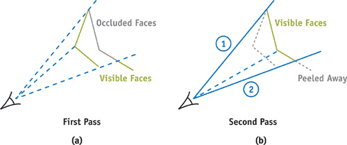
Figure 15-3 Two Possibilities When Peeling Away 3D Geometry
15.2.3 Composing Blueprints
We compose blueprints using visible and nonvisible edges stored in edge maps in depth-sorted order. For each edge map, we proceed as follows:
- We texture a screen-aligned quad that fills in the viewport with the edge map and its associated depth map.
- We further apply a fragment program that (1) performs depth sprite rendering using the appropriate depth layer map as input; (2) calculates the fragment's RGB value using the edge intensity value derived from accessing the edge map and, for instance, a bluish color; and (3) sets the fragment's alpha value to the edge intensity.
- We then use color blending by considering edge intensity values as blending factors for providing depth complexity cues while keeping edges enhanced.
We have found that in practice, it is sufficient to blend just the first few color layer maps to compose blueprints. The remaining layer maps have less visual impact on the overall composition because only a few (often isolated) pixels get colored. To alter the termination conditions for blueprint rendering and thus optimize rendering speed, we specify a desired minimal fraction of fragments (depending on the window resolution) to pass the depth test. In this way, we decrease the number of rendering passes while we maintain the visual quality of blueprints. To implement the trade-off between speed and quality, we configure the occlusion query extension appropriately. Figure 15-4a shows the resulting blueprint of the crank model.
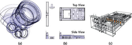
Figure 15-4 Various Applications of the Technique
15.2.4 Depth Masking
Depth masking is a technique that peels away a minimal number of depth layers until a specified fraction of a single, occluded component becomes visible. In fact, depth masking provides a termination condition for blueprint rendering to dynamically adapt the number of rendering passes. For depth masking, we proceed as follows:
- We derive a depth texture as the depth mask of the designated component in a preceding rendering pass.
- In successive rendering passes, we render the depth mask as a depth sprite whenever we have peeled away a depth layer. If a specified fraction of the number of fragments passes the ordinary depth test (based on the z-buffer contents just produced), we terminate our technique. Otherwise, we must peel away more depth layers.
- Finally, we simply integrate the designated component when composing blueprints.
The modifications to our technique are shown in pseudocode in Listing 15-2. Again, we use the occlusion query extension to implement the termination condition.
Example 15-2. Pseudocode with Modified Termination Condition to Implement Depth Masking
procedure depthPeeling(G 3DGeometry,
                       C geometryOfOccludedComponent) begin depthMask
    depthTexture(C)
quad createTexturedScreenAlignedQuad(depthMask) renderDepthSprite(quad)
    /* Render quad as depth sprite */
    int Q = occlusionQuery()
    /* Number of fragments of the components */
    ... do... renderDepthSprite(quad) int R = occlusionQuery()
    /* Number of visible fragments of the
    component */
    while (R < fraction(Q))
    /* Termination condition */
    end
15.2.5 Visualizing Architecture Using Blueprint Rendering
Blueprints can be used to outline the design of architecture. We apply blueprint rendering to generate plan views of architecture. Composing plan views using an orthographic camera is a straightforward task. In the visualization of the Temple of Ramses II in Abydos (Figure 15-4b), we can identify chambers, pillars, and statues systematically. Thus, blueprints increase the visual perception in these illustrations. The plan views are produced automatically.
A perspective view still provides better spatial orientation and conceptual insight in blueprints of architecture. Figure 15-4c visualizes the design of the entrance and the inner yard of the temple with its surrounding walls and statues. These are in front of the highlighted statues that guard the doorway to the rear part of the temple. With depth masking, we determine the number of depth layers that occlude the guarding statues and, therefore, must be peeled away. In this way, we can reduce the visual complexity of a blueprint if the structural complexity of the model is more than can be reasonably displayed.
15.3 Sketchy Rendering
Our sketchy drawing technique considers visually important edges and surface colors for sketching 3D geometry nonuniformly using uncertainty.
Our rendering technique proceeds as follows: As with blueprint rendering, we first generate intermediate rendering results that represent edges and surface colors of 3D geometry. Then we apply uncertainty values in image space to sketch these textures nonuniformly. Finally, we adjust depth information in such a way that the resulting sketchy drawing can be merged with general 3D scene contents.
15.3.1 Edges and Color Patches
We again use the edge enhancement technique to store edges of 3D geometry as an edge map for later usage, as shown in Figure 15-5a. In addition, we render surface colors of 3D geometry to texture to produce striking color patches that appear flat, cover all surface details, and emulate a cartoon-like style. We call that texture a shade map; see Figure 15-5b.
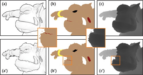
Figure 15-5 Applying Uncertainty Using Edge and Shade Maps
15.3.2 Applying Uncertainty
We apply uncertainty values to edges and surface colors in image space to simulate the effect of "sketching on a flat surface." For that purpose, we texture a screen-aligned quad (filling in the viewport of the canvas) using edge and shade maps as textures. Moreover, we apply an additional texture, whose texels represent uncertainty values. Because we want to achieve mostly continuous sketchy boundaries and frame-to-frame coherence, we opt for a noise texture whose texel values have been determined by the Perlin noise function (Perlin 1985); hence neighboring uncertainty values are correlated in image space. Once created (in a preprocessing step), the noise texture serves as an offset texture for accessing the edge and shade maps when rendering. That is, its texel values slightly perturb texture coordinates of each fragment of the quad that accesses the edge and shade maps.
In addition, we introduce a degree of uncertainty to control the amount of perturbation, for which we employ a user-defined 2 x 2 matrix. We multiply uncertainty values derived from the noise texture by that matrix to weight all these values uniformly and then use the resulting offset vector to translate the texture coordinates. Figure 15-6 illustrates the perturbation of the texture coordinates that access the shade map using the degree of uncertainty.
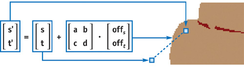
Figure 15-6 Applying Uncertainty in Image Space
To enhance the sketchiness effect, we perturb texture coordinates for accessing the edge and shade maps differently. We thus apply two different 2 x 2 matrices, resulting in different degrees of uncertainty for each map. One degree of uncertainty shifts texture coordinates of the edge map, and one shifts texture coordinates of the shade map—that is, we shift them in opposite directions. Figure 15-5 shows the edge and shade maps after we have applied uncertainty.
We denote texture values that correspond to fragments of 3D geometry as interior regions; texture values that do not correspond to fragments of 3D geometry are called exterior regions. So in conclusion, by texturing the quad and perturbing texture coordinates using uncertainty, we can access interior regions of the edge and shade maps, whereas the initial texture coordinates would access exterior regions and vice versa (Figure 15-6). In this way, interior regions can be sketched beyond the boundary of 3D geometry, and exterior regions can penetrate interior regions. We can even produce spots beyond the boundary of the 3D geometry (Figure 15-5).
Finally, we combine texture values of the edge and the shade maps. We multiply the intensity values derived from perturbing the edge map with the color values derived from perturbing the shade map. For the sketchy drawing in Figure 15-7a, we determined uncertainty values (offs , offt ) by using the turbulence function (based on Perlin noise):
offs turbulence(s, t);
and offt turbulence(1 - s, 1 - t);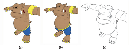
Figure 15-7 Different Styles of Sketchy Rendering
15.3.3 Adjusting Depth
Up to now, we have merely textured a screen-aligned quad with a sketchy depiction. This method has significant shortcomings. When we render the quad textured with textures of 3D geometry, (1) z-values of the original geometry are not present in interior regions, and in particular, (2) no z-values of the original geometry are present in exterior regions when uncertainty has been applied. Thus the sketchy rendering cannot correctly interact with other objects in the scene.
To overcome these shortcomings, we apply depth sprite rendering by considering previous perturbations. That is, we additionally texture the quad with the high-precision depth map (already available) and access this texture twice using perturbed texture coordinates. As first perturbation, we apply the degree of uncertainty used for accessing the edge map; as second perturbation, we apply the degree of uncertainty used for accessing the shade map. The minimum value of both these texture values produces the final z-value of the fragment for depth testing. Figure 15-5c' shows the result of both perturbations applied to the depth map. The interior region of the perturbed depth map matches the combination of the interior regions of both the perturbed edge map and the perturbed shade map. Even those spots produced for the shade map appear in the perturbation of the depth map.
Thus, modifying depth sprite rendering allows us to adjust z-values for the textured quad that represents a sketchy depiction of 3D geometry. So, the z-buffer remains in a correct state with respect to that geometry, and its sketchy representation can be composed with further (for example, nonsketchy) 3D geometry. The accompanying video on the book's CD illustrates this feature.
15.3.4 Variations of Sketchy Rendering
We present two variations of sketchy rendering, both of which also run in real time.
Roughened Profiles and Color Transitions
Although we sketch edges and surface colors nonuniformly, the profiles and the color transitions of a sketchy depiction are precise as if sketched with pencils on a flat surface. We roughen the profiles and color transitions to simulate different drawing tools and media, such as chalk applied on a rough surface. We apply randomly chosen noise values; hence, adjacent texture values of the noise texture are uncorrelated. Consequently, the degrees of uncertainty that we apply to the texture coordinates of adjacent fragments are also uncorrelated. In this way, we produce sketchy depictions with softened and frayed edges and color transitions, as shown in Figure 15-7b. The roughness and granularity, in particular for edges, vary as though the pressure had varied as it does when drawing with chalk. This effect depends on the amount of uncertainty that we apply in image space.
Repeated Edges
A fundamental technique in hand drawings is to repeatedly draw edges to draft a layout or design. We sketch visually important edges only to simulate this technique. For that purpose, we exclude the shade map but apply the edge map multiple times using different degrees of uncertainty and possibly different edge colors. Edges will then overlap nonuniformly as if the edges of the 3D geometry have been sketched repeatedly, as in Figure 15-7c. We also have to adjust the depth information by accessing the depth map multiple times, using the corresponding degrees of uncertainty.
15.3.5 Controlling Uncertainty
Controlling uncertainty values, in general, enables us to configure the visual appearance of sketchy renderings. By providing uncertainty values based on a Perlin noise function for each pixel in image space, (1) we achieve frame-to-frame coherence, for instance, when interacting with the scene (because neighboring uncertainty values are correlated), and (2) we can access interior regions from beyond exterior regions and, vice versa, sketch beyond the boundary of 3D geometries. However, uncertainty values remain unchanged in image space and have no obvious correspondence with geometric properties of the original 3D geometry. Consequently, sketchy drawings tend to "swim" in image space (known as the shower-door effect) and we cannot predetermine their visual appearance.
To overcome these limitations, we seek to accomplish the following:
- Preserve geometric properties such as surface positions, normals, or curvature information to determine uncertainty values.
- Continue to provide uncertainty values in exterior regions, at least close to the 3D geometry.
Preserving Geometric Properties
To preserve geometric properties of 3D geometry to control uncertainty, we proceed as follows:
- We render these geometric properties directly into a texture to generate an additional G-buffer.
- Next we texture the screen-aligned quad with that additional texture, and then access geometric properties using texture coordinates (s, t).
- Finally, we calculate uncertainty values based on a noise function, using the geometric properties as parameters.
Then we can use these uncertainty values to determine different degrees of uncertainty for perturbing texture coordinates resulting in (s', t'). Mathematically, we use the following function to determine the perturbed texture coordinates (s', t'):
|
f : (s, t)
|
|
f (s, t) = p(s, t, g(s, t)), |
 (s', t')
where (s, t) represent texture coordinates of a fragment produced when rasterizing the screen-aligned quad, g() provides the geometric properties available in the additional texture, and p() determines the perturbation applied to (s, t) using g() as input.
For sketchy rendering, we apply two functions f(s, t) to handle perturbations for the edge (fEdge (s, t)) and the shade (fShade (s, t)) maps differently.
Enlarging the Geometry
We enlarge the original 3D geometry to generate geometric properties in its surroundings in image space. We do this by slightly shifting each vertex of the mesh along its vertex normal in object space. For this technique to work as expected, the surface must at least form a connected component and each of its shared vertices must have an interpolated normal.
By enlarging the 3D geometry in this way, we can render the geometric properties into a texture for calculating uncertainty values in interior regions as well as in the exterior regions (nearby the original 3D geometry). That way, interior regions can be sketched beyond the boundary of the 3D geometry and exterior regions can penetrate interior regions. We can then apply perturbations based on uncertainty values that do have an obvious correspondence to the underlying 3D geometry.
15.3.6 Reducing the Shower-Door Effect
We now illustrate, by way of example, how to control sketchiness to reduce the shower-door effect for sketchy rendering.
We render enlarged 3D geometry with its object-space positions as color values into a texture. To do so, we determine the object-space positions for each of the displaced vertices and provide them as texture coordinates to the rasterization process. Then the rasterizer produces interpolated object-space positions for each fragment. A specialized fragment shader then outputs them as high-precision color values to a high-precision texture. Thus, g(s, t) preserves object-space positions.
Based on g(s, t), we can determine texture coordinates f (s, t) using p(). In our example, the function p() calculates the perturbation by a user-defined 2 x 2 matrix and by a Perlin noise function encoded into a 3D texture. Then we access the 3D texture using g(s, t) as texture coordinates. We multiply the resulting texture value by the 2 x 2 matrix to obtain a degree of uncertainty. The function f (s, t) then applies the degree of uncertainty to perturb (s, t), resulting in (s', t').
Calculating fEdge (s, t) and fShade (s, t) using different matrices results in the sketchy depiction in Figure 15-8. The accompanying video on the book's CD illustrates that the shower-door effect has been significantly reduced. The overview in Figure 15-8 illustrates the process flow of sketchy rendering by considering the underlying geometric properties.
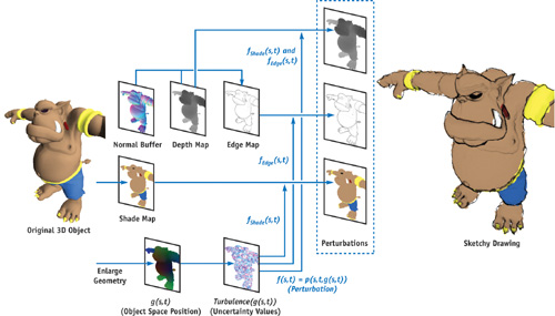
Figure 15-8 Buffers and Intermediate Rendering Results Involved in Sketchy Rendering
Although this example simply reduces the shower-door effect, it gives a clue as to how to control sketchy depictions using geometric properties. Using a higher-level shading language such as GLSL (Rost 2004) or Cg (Mark et al. 2003), one can further design and stylize sketchy drawings.
15.4 Conclusion
Blueprint rendering represents the first image-space rendering technique that renders visible and occluded edges of 3D geometries. In our future work, we aim at increasing visual perception of blueprints by combining edge maps based on techniques derived from volume rendering.
Sketchy drawing also represents the first image-space rendering technique that generates stylized edges of 3D geometries (Isenberg et al. 2003) for cartoon-like depictions. Because we produce and access the geometric properties and uncertainty values in exterior regions using intermediate rendering results, shaders written in higher-level shading languages alone are not enough to reproduce our technique for sketchy rendering. In our future work, we expect to reproduce artistically pleasing sketches.
15.5 References
Diefenbach, P. J. 1996. "Pipeline Rendering: Interaction and Realism Through Hardware-Based Multi-Pass Rendering." Ph.D. thesis. University of Pennsylvania.
Everitt, C. 2001. "Interactive Order-Independent Transparency." NVIDIA technical report. Available online at http://developer.nvidia.com/object/Interactive_Order_Transparency.html
Isenberg, T., B. Freudenberg, N. Halper, S. Schlechtweg, and T. Strothotte. 2003. "A Developer's Guide to Silhouette Algorithms for Polygonal Models." IEEE Computer Graphics and Applications 23(4), pp. 28–37.
Kilgard, M., ed. 2004. "NVIDIA OpenGL Extension Specifications." NVIDIA Corporation. Available online at http://www.nvidia.com/dev_content/nvopenglspecs/nvOpenGLspecs.pdf
Mark, W. R., R. S. Glanville, K. Akeley, and M. J. Kilgard. 2003. "Cg: A System for Programming Graphics Hardware in a C-like Language." ACM Transactions on Graphics (Proceedings of ACM SIGGRAPH 2003) 22(3), pp. 896–907.
Nienhaus, M., and J. Döllner. 2003. "Edge-Enhancement: An Algorithm for Real-Time Non-Photorealistic Rendering." Journal of WSCG '03, pp. 346–353.
Perlin, K. 1985. "An Image Synthesizer." In Computer Graphics (Proceedings of SIGGRAPH 85) 19(3), pp. 287–296.
Rost, R. J. 2004. OpenGL Shading Language. Addison-Wesley.
Saito, T., and T. Takahashi. 1990. "Comprehensible Rendering of 3-D Shapes." In Computer Graphics (Proceedings of SIGGRAPH 90) 24(4), August 1990, pp. 197–206.
The authors want to thank ART+COM, Berlin, for providing the model of the Temple of Ramses II; Amy and Bruce Gooch for the crank model; and Konstantin Baumann, Johannes Bohnet, Henrik Buchholz, Oliver Kersting, Florian Kirsch, and Stefan Maass for their contributions to the Virtual Rendering System.
Copyright
Many of the designations used by manufacturers and sellers to distinguish their products are claimed as trademarks. Where those designations appear in this book, and Addison-Wesley was aware of a trademark claim, the designations have been printed with initial capital letters or in all capitals.
The authors and publisher have taken care in the preparation of this book, but make no expressed or implied warranty of any kind and assume no responsibility for errors or omissions. No liability is assumed for incidental or consequential damages in connection with or arising out of the use of the information or programs contained herein.
NVIDIA makes no warranty or representation that the techniques described herein are free from any Intellectual Property claims. The reader assumes all risk of any such claims based on his or her use of these techniques.
The publisher offers excellent discounts on this book when ordered in quantity for bulk purchases or special sales, which may include electronic versions and/or custom covers and content particular to your business, training goals, marketing focus, and branding interests. For more information, please contact:
U.S. Corporate and Government Sales
(800) 382-3419
corpsales@pearsontechgroup.com
For sales outside of the U.S., please contact:
International Sales
international@pearsoned.com
Visit Addison-Wesley on the Web: www.awprofessional.com
Library of Congress Cataloging-in-Publication Data
GPU gems 2 : programming techniques for high-performance graphics and general-purpose
computation / edited by Matt Pharr ; Randima Fernando, series editor.
p. cm.
Includes bibliographical references and index.
ISBN 0-321-33559-7 (hardcover : alk. paper)
1. Computer graphics. 2. Real-time programming. I. Pharr, Matt. II. Fernando, Randima.
T385.G688 2005
006.66—dc22
2004030181
GeForce™ and NVIDIA Quadro® are trademarks or registered trademarks of NVIDIA Corporation.
Nalu, Timbury, and Clear Sailing images © 2004 NVIDIA Corporation.
mental images and mental ray are trademarks or registered trademarks of mental images, GmbH.
Copyright © 2005 by NVIDIA Corporation.
All rights reserved. No part of this publication may be reproduced, stored in a retrieval system, or transmitted, in any form, or by any means, electronic, mechanical, photocopying, recording, or otherwise, without the prior consent of the publisher. Printed in the United States of America. Published simultaneously in Canada.
For information on obtaining permission for use of material from this work, please submit a written request to:
Pearson Education, Inc.
Rights and Contracts Department
One Lake Street
Upper Saddle River, NJ 07458
Text printed in the United States on recycled paper at Quebecor World Taunton in Taunton, Massachusetts.
Second printing, April 2005
Dedication
To everyone striving to make today's best computer graphics look primitive tomorrow
- Copyright
- Inside Back Cover
- Inside Front Cover
- Part I: Geometric Complexity
-
- Chapter 1. Toward Photorealism in Virtual Botany
- Chapter 2. Terrain Rendering Using GPU-Based Geometry Clipmaps
- Chapter 3. Inside Geometry Instancing
- Chapter 4. Segment Buffering
- Chapter 5. Optimizing Resource Management with Multistreaming
- Chapter 6. Hardware Occlusion Queries Made Useful
- Chapter 7. Adaptive Tessellation of Subdivision Surfaces with Displacement Mapping
- Chapter 8. Per-Pixel Displacement Mapping with Distance Functions
- Part II: Shading, Lighting, and Shadows
-
- Chapter 9. Deferred Shading in S.T.A.L.K.E.R.
- Chapter 10. Real-Time Computation of Dynamic Irradiance Environment Maps
- Chapter 11. Approximate Bidirectional Texture Functions
- Chapter 12. Tile-Based Texture Mapping
- Chapter 13. Implementing the mental images Phenomena Renderer on the GPU
- Chapter 14. Dynamic Ambient Occlusion and Indirect Lighting
- Chapter 15. Blueprint Rendering and "Sketchy Drawings"
- Chapter 16. Accurate Atmospheric Scattering
- Chapter 17. Efficient Soft-Edged Shadows Using Pixel Shader Branching
- Chapter 18. Using Vertex Texture Displacement for Realistic Water Rendering
- Chapter 19. Generic Refraction Simulation
- Part III: High-Quality Rendering
-
- Chapter 20. Fast Third-Order Texture Filtering
- Chapter 21. High-Quality Antialiased Rasterization
- Chapter 22. Fast Prefiltered Lines
- Chapter 23. Hair Animation and Rendering in the Nalu Demo
- Chapter 24. Using Lookup Tables to Accelerate Color Transformations
- Chapter 25. GPU Image Processing in Apple's Motion
- Chapter 26. Implementing Improved Perlin Noise
- Chapter 27. Advanced High-Quality Filtering
- Chapter 28. Mipmap-Level Measurement
- Part IV: General-Purpose Computation on GPUS: A Primer
-
- Chapter 29. Streaming Architectures and Technology Trends
- Chapter 30. The GeForce 6 Series GPU Architecture
- Chapter 31. Mapping Computational Concepts to GPUs
- Chapter 32. Taking the Plunge into GPU Computing
- Chapter 33. Implementing Efficient Parallel Data Structures on GPUs
- Chapter 34. GPU Flow-Control Idioms
- Chapter 35. GPU Program Optimization
- Chapter 36. Stream Reduction Operations for GPGPU Applications
- Part V: Image-Oriented Computing
-
- Chapter 37. Octree Textures on the GPU
- Chapter 38. High-Quality Global Illumination Rendering Using Rasterization
- Chapter 39. Global Illumination Using Progressive Refinement Radiosity
- Chapter 40. Computer Vision on the GPU
- Chapter 41. Deferred Filtering: Rendering from Difficult Data Formats
- Chapter 42. Conservative Rasterization
- Part VI: Simulation and Numerical Algorithms
-
- Chapter 43. GPU Computing for Protein Structure Prediction
- Chapter 44. A GPU Framework for Solving Systems of Linear Equations
- Chapter 45. Options Pricing on the GPU
- Chapter 46. Improved GPU Sorting
- Chapter 47. Flow Simulation with Complex Boundaries
- Chapter 48. Medical Image Reconstruction with the FFT