
GPU Gems 2
GPU Gems 2 is now available, right here, online. You can purchase a beautifully printed version of this book, and others in the series, at a 30% discount courtesy of InformIT and Addison-Wesley.
The CD content, including demos and content, is available on the web and for download.
Chapter 33. Implementing Efficient Parallel Data Structures on GPUs
Aaron Lefohn
University of California, Davis
Joe Kniss
University of Utah
John Owens
University of California, Davis
Modern GPUs, for the first time in computing history, put a data-parallel, streaming computing platform in nearly every desktop and notebook computer. A number of recent academic research papers—as well as other chapters in this book—demonstrate that these streaming processors are capable of accelerating a much broader scope of applications than the real-time rendering applications for which they were originally designed. Leveraging this computational power, however, requires using a fundamentally different programming model that is foreign to many programmers. This chapter seeks to demystify one of the most fundamental differences between CPU and GPU programming: the memory model. Unlike traditional CPU-based programs, GPU-based programs have a number of limitations on when, where, and how memory can be accessed. This chapter gives an overview of the GPU memory model and explains how fundamental data structures such as multidimensional arrays, structures, lists, and sparse arrays are expressed in this data-parallel programming model.
33.1 Programming with Streams
Modern graphics processors are now capable of accelerating much more than real-time computer graphics. Recent work in the emerging field of general-purpose computation on graphics processing units (GPGPU) has shown that GPUs are capable of accelerating applications as varied as fluid dynamics, advanced image processing, photorealistic rendering, and even computational chemistry and biology (Buck et al. 2004, Harris et al. 2004). The key to using the GPU for purposes other than real-time rendering is to view it as a streaming, data-parallel computer (see Chapter 29 in this book, "Streaming Architectures and Technology Trends," as well as Dally et al. 2004). The way in which we structure computation and access memory in GPU programs is greatly influenced by this stream computation model. As such, we first give a brief overview of this model before discussing GPU-based data structures.
Streaming processors such as GPUs are programmed in a fundamentally different way than serial processors like today's CPUs. Most programmers are familiar with a programming model in which they can write to any location in memory at any point in their program. When programming a streaming processor, in contrast, we access memory in a much more structured manner. In the stream model, programs are expressed as series of operations on data streams, as shown in Figure 33-1. The elements in a stream (that is, an ordered array of data) are processed by the instructions in a kernel (that is, a small program). A kernel operates on each element of a stream and writes the results to an output stream.
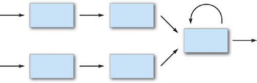
Figure 33-1 Stream Program as Data-Dependency Graph
The stream programming model restrictions allow GPUs to execute kernels in parallel and therefore process many data elements simultaneously. This data parallelism is made possible by ensuring that the computation on one stream element cannot affect the computation on another element in the same stream. Consequently, the only values that can be used in the computation of a kernel are the inputs to that kernel and global memory reads. In addition, GPUs require that the outputs of kernels be independent: kernels cannot perform random writes into global memory (in other words, they may write only to a single stream element position of the output stream). The data parallelism afforded by this model is fundamental to the speedup offered by GPUs over serial processors.
Following are two sample snippets of code showing how to transform a serial program into a data-parallel stream program. The first sample shows a loop over an array (for example, the pixels in an image) for a serial processor. Note that the instructions in the loop body are specified for only a single data element at a time:
for (i = 0; i < data.size(); i++)
loopBody(data[i])
The next sample shows the same section of code written in pseudocode for a streaming processor:
inDataStream = specifyInputData() kernel = loopBody() outDataStream =
    apply(kernel, inDataStream)
The first line specifies the data stream. In the case of our image example, the stream is all of the pixels in the image. The second line specifies the computational kernel, which is simply the body of the loop from the first sample. Lastly, the third line applies the kernel to all elements in the input stream and stores the results in an output stream. In the image example, this operation would process the entire image and produce a new, transformed image.
Current GPU fragment processors have an additional programming restriction beyond the streaming model described earlier. Current GPU fragment processors are single-instruction, multiple-data (SIMD) parallel processors. This has traditionally meant that all stream elements (that is, fragments) must be processed by the same sequence of instructions. Recent GPUs (those supporting Pixel Shader 3.0 [Microsoft 2004a]) relax this strict SIMD model slightly by allowing variable-length loops and limited fragment-level branching. The hardware remains fundamentally SIMD, however, and thus branching must be spatially coherent between fragments for efficient execution (see Chapter 34 in this book, "GPU Flow-Control Idioms," for more information). Current vertex processors (Vertex Shader 3.0 [Microsoft 2004b]) are multiple-instruction, multiple-data (MIMD) machines, and can therefore execute kernel branches more efficiently than fragment processors. Although less flexible, the fragment processor's SIMD architecture is highly efficient and cost-effective.
Because nearly all GPGPU computations are currently performed with the more powerful fragment processor, GPU-based data structures must fit into the fragment processor's streaming, SIMD programming model. Therefore, all data structures in this chapter are expressed as streams, and the computations on these data structures are in the form of SIMD, data-parallel kernels.
33.2 The GPU Memory Model
Graphics processors have their own memory hierarchy analogous to the one used by serial microprocessors, including main memory, caches, and registers. This memory hierarchy, however, is designed for accelerating graphics operations that fit into the streaming programming model rather than general, serial computation. Moreover, graphics APIs such as OpenGL and Direct3D further limit the use of this memory to graphics-specific primitives such as vertices, textures, and frame buffers. This section gives an overview of the current memory model on GPUs and how stream-based computation fits into it.
33.2.1 Memory Hierarchy
Figure 33-2 shows the combined CPU and GPU memory hierarchy. The GPU's memory system creates a branch in a modern computer's memory hierarchy. The GPU, just like a CPU, has its own caches and registers to accelerate data access during computation. GPUs, however, also have their own main memory with its own address space—meaning that programmers must explicitly copy data into GPU memory before beginning program execution. This transfer has traditionally been a bottleneck for many applications, but the advent of the new PCI Express bus standard may make sharing memory between the CPU and GPU a more viable possibility in the near future.
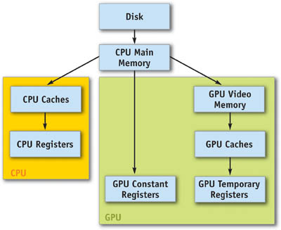
Figure 33-2 The CPU and GPU Memory Hierarchies
33.2.2 GPU Stream Types
Unlike CPU memory, GPU memory has a number of usage restrictions and is accessible only via the abstractions of a graphics programming interface. Each of these abstractions can be thought of as a different stream type with its own set of access rules. The three types of streams visible to the GPU programmer are vertex streams, frame-buffer streams, and texture streams. A fourth stream type, fragment streams, is produced and consumed entirely within the GPU. Figure 33-3 shows the pipeline for a modern GPU, the three user-accessible streams, and the points in the pipeline where each can be used.
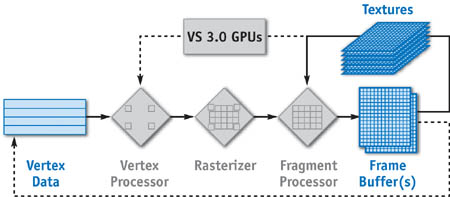
Figure 33-3 Streams in Modern GPUs
Vertex Streams
Vertex streams are specified as vertex buffers via the graphics API. These streams hold vertex positions and a variety of per-vertex attributes. These attributes have traditionally been used for texture coordinates, colors, normals, and so on, but they can be used for arbitrary input stream data for vertex programs.
Vertex programs are not allowed to randomly index into their input vertices. Until recently, vertex streams could be updated only by transferring data from the CPU to the GPU. The GPU was not allowed to write to vertex streams. Recent API enhancements, however, have made it possible for the GPU to write to vertex streams. This is accomplished by either "copy-to-vertex-buffer" or "render-to-vertex-buffer." In the former technique, rendering results are copied from a frame buffer to a vertex buffer; in the latter technique, the rendering results are written directly to a vertex buffer. The recent addition of GPU-writable vertex streams enables GPUs, for the first time, to loop stream results from the end to the beginning of the pipeline.
Fragment Streams
Fragment streams are generated by the rasterizer and consumed by the fragment processor. They are the stream inputs to fragment programs, but they are not directly accessible to programmers because they are created and consumed entirely within the graphics processor. Fragment stream values include all of the interpolated outputs from the vertex processor: position, color, texture coordinates, and so on. As with per-vertex stream attributes, the per-fragment values that have traditionally been used for texture coordinates may now be used for any stream value required by the fragment program.
Fragment streams cannot be randomly accessed by fragment programs. Permitting random access to the fragment stream would create a dependency between fragment stream elements, thus breaking the data-parallel guarantee of the programming model. If random access to fragment streams is needed by algorithms, the stream must first be saved to memory and converted to a texture stream.
Frame-Buffer Streams
Frame-buffer streams are written by the fragment processor. They have traditionally been used to hold pixels for display to the screen. Streaming GPU computation, however, uses frame buffers to hold the results of intermediate computation stages. In addition, modern GPUs are able to write to multiple frame-buffer surfaces (that is, multiple RGBA buffers) simultaneously. Current GPUs can write up to 16 floating-point scalar values per render pass (this value is expected to increase in future hardware).
Frame-buffer streams cannot be randomly accessed by either fragment or vertex programs. They can, however, be directly read from or written to by the CPU via the graphics API. Lastly, recent API enhancements have begun to blur the distinction between frame buffers, vertex buffers, and textures by allowing a render pass to be directly written to any of these stream types.
Texture Streams
Textures are the only GPU memory that is randomly accessible by fragment programs and, for Vertex Shader 3.0 GPUs, vertex programs. If programmers need to randomly index into a vertex, fragment, or frame-buffer stream, they must first convert it to a texture. Textures can be read from and written to by either the CPU or the GPU. The GPU writes to textures either by rendering directly to them instead of to a frame buffer or by copying data from a frame buffer to texture memory.
Textures are declared as 1D, 2D, or 3D streams and addressed with a 1D, 2D, or 3D address, respectively. A texture can also be declared as a cube map, which can be treated as an array of six 2D textures.
33.2.3 GPU Kernel Memory Access
Vertex and fragment programs (kernels) are the workhorses of modern GPUs. Vertex programs operate on vertex stream elements and send output to the rasterizer. Fragment programs operate on fragment streams and write output to frame buffers. The capabilities of these programs are defined by the arithmetic operations they can perform and the memory they are permitted to access. The variety of available arithmetic operations permitted in GPU kernels is approaching those available on CPUs, yet there are numerous memory access restrictions. As described previously, many of these restrictions are in place to preserve the parallelism required for GPUs to maintain their speed advantage. Other restrictions, however, are artifacts of the evolving GPU architecture and will almost certainly be relaxed in future generations.
The following is a list of memory access rules for vertex and fragment kernels on GPUs that support Pixel Shader 3.0 and Vertex Shader 3.0 functionality (Microsoft 2004a, b):
- No CPU main memory access; no disk access.
- No GPU stack or heap.
- Random reads from global texture memory.
- Reads from constant registers.
- - Vertex programs can use relative indexing of constant registers.
- Reads/writes to temporary registers.
- - Registers are local to the stream element being processed.
- - No relative indexing of registers.
- Streaming reads from stream input registers.
- - Vertex kernels read from vertex streams.
- - Fragment kernels read from fragment streams (rasterizer results).
- Streaming writes (at end of kernel only).
-
- Write location is fixed by the position of the element in the stream.
Cannot write to computed address (that is, no scatter).
-
- Vertex kernels write to vertex output streams.
Can write up to 12 four-component floating-point values.
-
- Fragment kernels write to frame-buffer streams.
Can write up to 4 four-component floating-point values.
-
An additional access pattern emerges from the preceding set of rules and the stream types described in Section 33.2.2: pointer streams (Purcell et al. 2002). Pointer streams arise out of the ability to use any input stream as the address for a texture read. Figure 33-4 shows that pointer streams are simply streams whose values are memory addresses. If the pointer stream is read from a texture, this capability is called dependent texturing.
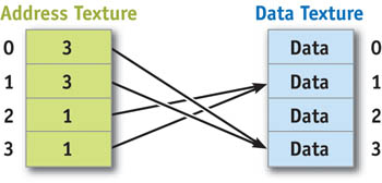
Figure 33-4 Implementing Pointer Streams with Textures
33.3 GPU-Based Data Structures
While the previous sections have described the GPU and its programming model with elegant abstractions, we now delve into the details of real-world data structures on current GPUs. The abstractions from Sections 33.1 and 33.2 continue to apply to the data structures herein, but the architectural restrictions of current GPUs make the real-world implementations slightly more complicated.
We first describe implementations of basic structures: multidimensional arrays and structures. We then move on to more advanced structures in Sections 33.3.3 and 33.3.4: static and dynamic sparse structures.
33.3.1 Multidimensional Arrays
Why include a section about multidimensional arrays if the GPU already provides 1D, 2D, and 3D textures? There are two reasons. First, current GPUs provide only 2D rasterization and 2D frame buffers. This means the only kind of texture that can be easily updated is a 2D texture, because it is a natural replacement for a 2D frame buffer. [1] Second, textures currently have restrictions on their size in each dimension. For example, current GPUs do not support 1D textures with more than 4,096 elements. If GPUs could write to an N-D frame buffer (where N = 1, 2, 3, . . .) with no size restrictions, this section would be trivial.
Given these restrictions, 2D textures with nearest-neighbor filtering are the substrate on which nearly all GPGPU-based data structures are built. [2] Note that until recently, the size of each texture dimension was required to be a power of two, but this restriction is thankfully no longer in place.
All of the following examples use address translation to convert an N-D array address into a 2D texture address. Although it is important to minimize the cost of this address translation, remember that CPU-based multidimensional arrays must also perform address translation to look up values in the underlying 1D array. In fact, the GPU's texture-addressing hardware actually helps make these translations very efficient. Current GPUs do, however, suffer from one problem related to these address translations: the limitations of floating-point addressing. Chapter 32 of this book discusses important limitations and errors associated with using floating-point rather than integer addresses, and those problems apply to the techniques presented in this section.
1D Arrays
One-dimensional arrays are represented by packing the data into a 2D texture, as shown in Figure 33-5. Current GPUs can therefore represent 1D arrays containing up to 16,777,216 (4,096x4,096) elements. [3] Each time this packed array is accessed from a fragment or vertex program, the 1D address must be converted to a 2D texture coordinate.
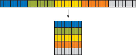
Figure 33-5 1D Arrays Packed into 2D Arrays
Two versions of this address translation are shown in Cg syntax in Listings 33-1 and 33-2. Listing 33-1 (Buck et al. 2004) shows code for using rectangle textures, which use integer addresses and do not support repeat-tiling address modes. Note that CONV_CONST is a constant based on the texture size and should be precomputed rather than recomputed for each stream element. Section 33.4 describes an elegant technique for computing values such as CONV_CONST with a feature of the Cg compiler called program specialization. With this optimization, Listing 33-1 compiles to three assembly instructions.
Example 33-1. 1D to 2D Address Translation for Integer-Addressed Textures
float2 addrTranslation_1DtoRECT(float address1D, float2 texSize)
{
  // Parameter explanation:
  // - "address1D" is a 1D array index into an array of size N
  // - "texSize" is size of RECT texture that stores the 1D array
  // Step 1) Convert 1D address from [0,N] to [0,texSize.y]
  float CONV_CONST = 1.0 / texSize.x;
  float normAddr1D = address1D * CONV_CONST;
  // Step 2) Convert the [0,texSize.y] 1D address to 2D.
  // Performing Step 1 first allows us to efficiently compute the
  // 2D address with "frac" and "floor" instead of modulus
  // and divide. Note that the "floor" of the y-component is
  // performed by the texture system.
  float2 address2D = float2(frac(normAddr1D) * texSize.x, normAddr1D);
  return address2D;
}
Listing 33-2 shows an address translation routine that can be used with traditional 2D textures, which use normalized [0,1] addressing. If CONV_CONST is precomputed, this address translation takes two fragment assembly instructions. It may also be possible to eliminate the frac instruction from Listing 33-2 by using the repeating-tiled addressing mode (such as GL_REPEAT). This reduces the conversion to a single assembly instruction. This optimization may be problematic on some hardware and texture configurations, however, so it should be carefully tested on your target architecture.
2D Arrays
Two-dimensional arrays are represented simply as 2D textures. Their maximum size is limited by the GPU driver. That limit for current GPUs ranges from 2048x2048 to 4096x4096 depending on the display driver and the GPU. These limits can be queried via the graphics API.
Example 33-2. 1D to 2D Address Translation for Normalized-Addressed Textures
float2 addrTranslation_1Dto2D(float address1D, float2 texSize)
{
  // Parameter explanation:
  // - "address1D" is a 1D array index into an array of size N
  // - "texSize" is size of 2D texture that stores the 1D array
  // NOTE: Precompute CONV_CONST before running the kernel.
float2 CONV_CONST = float2( 1.0 / texSize.x,
1.0 / (texSize.x * texSize.y );
// Return a normalized 2D address (with values in [0,1])
float2 normAddr2D = address1D * CONV_CONST;
float2 address2D = float2( frac(normAddr2D.x), normAddr2D.y );
return address2D;
}
3D Arrays
Three-dimensional arrays may be stored in one of three ways: in a 3D texture, with each slice stored in a separate 2D texture, or packed into a single 2D texture (Harris et al. 2003, Lefohn et al. 2003, Goodnight et al. 2003). Each of these techniques has pros and cons that affect the best representation for an application.
The simplest approach, using a 3D texture, has two distinct advantages. The first is that no address translation computation is required to access the memory. The second advantage is that the GPU's native trilinear filtering may be used to easily create high-quality volume renderings of the data. A disadvantage is that GPUs can update at most only four slices of the volume per render pass—thus requiring many passes to write to the entire array.
The second solution is to store each slice of the 3D texture in a separate 2D texture, as shown in Figure 33-6. The advantages are that, like a native 3D representation, no address translation is required for data access, and yet each slice can be easily updated without requiring render-to-slice-of-3D-texture API support. The disadvantage is that the volume can no longer be truly randomly accessed, because each slice is a separate texture. The programmer must know which slice numbers will be accessed before the kernel executes, because fragment and vertex programs cannot dynamically compute which texture to access at runtime.
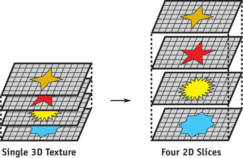
Figure 33-6 Storing a 3D Texture with Separate 2D Slices
The third option is to pack the 3D array into a single 2D texture, as shown in Figure 33-7. This solution requires an address translation for each data access, but the entire 3D array can be updated in a single render pass and no render-to-slice-of-3D-texture functionality is required. The ability to update the entire volume in a single render pass may have significant performance benefits, because the GPU's parallelism is better utilized when processing large streams. Additionally, unlike the 2D slice layout, the entire 3D array can be randomly accessed from within a kernel.
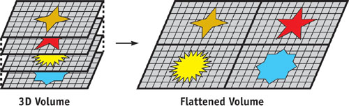
Figure 33-7 3D Arrays Flattened into a Single 2D Texture
A disadvantage of both the second and third schemes is that the GPU's native trilinear filtering cannot be used for high-quality volume rendering of the data. Fortunately, alternate volume rendering algorithms can efficiently render high-quality, filtered images from these complex 3D texture formats (see Chapter 41 of this book, "Deferred Filtering: Rendering from Difficult Data Formats").
The Cg code in Listing 33-3 shows one form of address translation to convert a 3D address into a 2D address for a packed representation. This packing is identical to the one used for the 1D arrays in Listings 33-1 and 33-2. It simply converts the 3D address to a large 1D address space before packing the 1D space into a 2D texture. This packing scheme was presented in Buck et al. 2004. Note that this scheme can use either of the conversions shown in Listing 33-1 and 33-2, depending on the type of the data texture (2D or rectangle).
Example 33-3. Converting a 3D Address into a 2D Address
float2 addrTranslation_3Dto2D(float3 address3D, float3 sizeTex3D,
                              float2 sizeTex2D)
{
  // Parameter explanation:
  // - "address3D" is 3D array index into a 3D array of "sizeTex3D"
  // - "sizeTex2D" is size of 2D texture that stores the 3D array
  // Step 1) Texture size constant (This should be precomputed!)
  float3 SIZE_CONST = float3(1.0, sizeTex3D.x, sizeTex3D.y * sizeTex3D.x);
  // Step 2) Convert 3D address to 1D address in [0, sizeTex2D.y]
  float address1D = dot(address3D, SIZE_CONST);
  // Step 3) Convert [0, texSize.y] 1D address to 2D using the
  // 1D-to-2D translation function defined in Listing 33-1.
  return addrTranslation_1Dto2D(address1D, sizeTex2D);
}
The Cg code for a slice-based, alternate packing scheme is shown in Listing 33-4. This scheme packs slices of the 3D texture into the 2D texture. One difficulty in this scheme is that the width of the 2D texture must be evenly divisible by the width of a slice of the 3D array. The advantage is that native bilinear filtering may be used within each slice. Note that the entire address translation reduces to two instructions (a 1D texture lookup and a multiply-add) if the sliceAddr computation is stored in a 1D lookup table texture indexed by address3D.z and nSlicesPerRow is precomputed.
Example 33-4. Source Code for Packing Slices of 3D Texture in a 2D Texture
float2 addrTranslation_slice_3Dto2D(float3 address3D, float3 sizeTex3D,
                                    float2 sizeTex2D)
{
  // NOTE: This should be precomputed
  float nSlicesPerRow = sizeTex2D.x / sizeTex3D.x;
  // Compute (x,y) for slice in address space of the slices
  float2 sliceAddr = float2(fmod(address3D.z, nSlicesPerRow),
                            floor(address3D.z / nSlicesPerRow));
  // Convert sliceSpace address to 2D texture address
  float2 sliceSize = float2(address3D.x, address3D.y);
  float2 offset = sliceSize * sliceAddr;
  return addr3D.xy + offset;
}
Note that there would be no reason to store 3D arrays in 2D textures if GPUs supported either 3D rasterization with 3D frame buffers or the ability to "cast" textures from 2D to 3D. In the latter case, the GPU would rasterize the 2D, flattened form of the array but allow the programmer to read from it using 3D addresses.
Higher-Dimensional Arrays
Higher-dimensional arrays can be packed into 2D textures using a generalized form of the packing scheme shown in Listing 33-3 (Buck et al. 2004).
33.3.2 Structures
A "stream of structures" such as the one shown in Listing 33-5 must be defined instead as a "structure of streams," as shown in Listing 33-6. In this construct, a separate stream is created for each structure member. In addition, the structures may not contain more data than can be output per fragment by the GPU. [4] These restrictions are due to the inability of fragment programs to specify the address to which their frame-buffer result is written (that is, they cannot perform a scatter operation). By specifying structures as a "structure of streams," each structure member has the same stream index, and all members can therefore be updated by a single fragment program.
Example 33-5. Stream of Structures
// WARNING: "Streams of structures" like the one shown
// in this example cannot be easily updated on current GPUs.
struct Foo
{
  float4 a;
  float4 b;
};
// This "stream of structures" is problematic
Foo foo[N];
Example 33-6. Structure of Streams
// This "structure of streams" can be easily updated on
// current GPUs if the number of data members in each structure
// is <= the number of fragment outputs supported by the GPU.
struct Foo
{
  float4 a[N];
  float4 b[N];
};
// Define a separate stream for each member
float4 Foo_a[N];
float4 Foo_b[N];
33.3.3 Sparse Data Structures
The arrays and structures we've discussed thus far are dense structures. In other words, all elements in the address space of the arrays contain valid data. There are many problems, however, whose efficient solution requires sparse data structures (such as lists, trees, or sparse matrices). Sparse data structures are an important part of many optimized CPU-based algorithms; brute-force GPU-based implementations that use dense data structures in their place are often slower than their optimized CPU counterparts. In addition, sparse data structures can reduce an algorithm's memory requirement—an important consideration given the limited amount of available GPU memory.
Despite their importance, GPU implementations of sparse data structures are problematic. The first reason is that updating sparse structures usually involves writing to a computed memory address (that is, scattering). The second difficulty is that traversing a sparse structure often involves a nonuniform number of pointer dereferences to access the data. This is problematic because, as discussed in Section 33.1, current fragment processors are SIMD machines that must process coarse batches of stream elements with exactly the same instructions. Researchers have nonetheless recently shown that a number of sparse structures can be implemented with current GPUs.
Static Sparse Structures
We begin by describing static GPU-based sparse data structures whose structure does not change during GPU computation. Examples of such data structures include the list of triangles in Purcell's ray acceleration grid (Purcell et al. 2002) and the sparse matrices in Bolz et al. 2003 and Krüger and Westermann 2003. In these structures, the location and number of sparse elements are fixed throughout the GPU computation. For example, the location and number of triangles in the ray-traced scene do not change. Because the structures are static, they do not have to write to computed memory addresses.
All of these structures use one or more levels of indirection to represent the sparse structures in memory. Purcell's ray acceleration structure, for example, begins with a regular 3D grid of triangle list pointers, as shown in Figure 33-8. The 3D grid texture contains a pointer to the start of the triangle list (stored in a second texture) for that grid cell. Each entry in the triangle list, in turn, contains a pointer to vertex data stored in a third texture. Similarly, the sparse matrix structures use a fixed number of levels of indirection to find nonzero matrix elements.
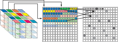
Figure 33-8 Purcell's Sparse Ray-Tracing Data Structure
These structures solve the problem of irregular access patterns with one of two different methods. The first method is to break the structure into blocks, where all elements in the block have an identical access pattern and can therefore be processed together. The second method is to have each stream element process one item from its list per render pass. Those elements with more items to process will continue to compute results, while those that have reached the end of their list will be disabled. [5]
An example of the blocking strategy is found in Bolz et al. 2003. They split sparse matrices into blocks that have the same number of nonzero elements and pad similar rows so that they have identical layouts. The algorithm for traversing the triangle lists found in Purcell et al. 2002 is an example of nonuniform traversal via conditional execution. All active rays (stream elements) process one element from their respective lists in each render pass. Rays become inactive when they reach the end of their triangle list, while rays that have more triangles to process continue to execute.
Note that the constraint of uniform access patterns for all stream elements is a restriction of the SIMD execution model of current GPUs. If future GPUs support MIMD stream processing, accessing irregular sparse data structures may become much easier. For example, the limited branching offered in Pixel Shader 3.0 GPUs already offers more options for data structure traversal than previous GPU generations.
Dynamic Sparse Structures
GPU-based sparse data structures that are updated during a GPU computation are an active area of research. Two noteworthy examples are the photon map in Purcell et al. 2003 and the deformable implicit surface representation in Lefohn et al. 2003, 2004. This section gives a brief overview of these data structures and the techniques used to update them.
A photon map is a sparse, adaptive data structure used to estimate the irradiance (that is, the light reaching a surface) in a scene. Purcell et al. (2003) describe an entirely GPU-based photon map renderer. To create the photon map on the GPU, they devise two schemes for writing data to computed memory addresses (that is, scatter) on current GPUs. The first technique computes the memory addresses and the data to be stored at those addresses. It then performs the scatter by performing a data-parallel sort operation on these buffers. The second technique, stencil routing, uses the vertex processor to draw large points at positions defined by the computed memory addresses. It resolves conflicts (when two data elements are written to the same address) via an ingenious stencil-buffer trick that routes data values to unique bins (pixel locations) even when they are drawn at the same fragment position. The nonuniform data are accessed in a manner similar to the triangle list traversal described in the previous subsection.
Another GPU-based dynamic sparse data structure is the sparse volume structure used for implicit surface deformation by Lefohn et al. (2003, 2004). An implicit surface defines a 3D surface as an isosurface (or level set) of a volume. A common example of 2D isosurfaces is the contour lines drawn on topographic maps. A contour line comprises points on the map that have the same elevation. Similarly, an implicit 3D surface is an isosurface of the scalar values stored in a volume's voxels. Representing surfaces in this way is very convenient from a mathematical standpoint, allowing the surface to freely distort and change topology.
Efficient representations of implicit surfaces use a sparse data structure that stores only the voxels near the surface rather than the entire volume, as shown in Figure 33-9. Lefohn et al. (2003, 2004) describe a GPU-based technique for deforming implicit surfaces from one shape into another. As the surface evolves, the sparse data structure representing it must also evolve (because the size of the data structure is proportional to the surface area of the implicit surface). For example, if the initial surface is a small sphere and the final form is a large square, the final form will require significantly more memory than was required for the initial sphere. The remainder of this section describes this sparse volume structure and how it evolves with the moving surface.
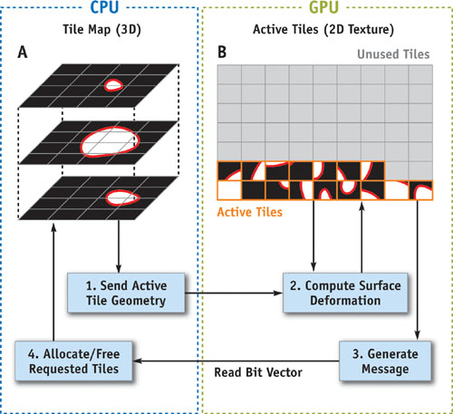
Figure 33-9 Dynamic Sparse Volume Data on the GPU
The sparse structure is created by subdividing the 3D volume into small 2D tiles (see the section marked "A" in Figure 33-9). The CPU stores tiles that contain the surface (that is, active tiles) in GPU texture memory (see the section marked "B" in Figure 33-9). The GPU performs the surface deformation computation on only the active tiles (see step 2 in Figure 33-9). The CPU keeps a map of the active tiles and allocates/frees tiles as necessary for the GPU computation. This scheme solves the dynamic update problem by employing the CPU as a memory management coprocessor for the GPU.
A key component of the system is the way in which the GPU requests that the CPU allocate or free tiles. The CPU receives the communication by reading a small encoded message (image) from the GPU (see steps 3 and 4 in Figure 33-9). This image contains one pixel per active tile, and the value of each pixel is a bit code. The 7-bit code has 1 bit for the active tile and 6 bits for each of the tiles neighboring it in the 3D volume. The value of each bit instructs the CPU to allocate or free the associated tile. The CPU, in fact, interprets the entire image as a single bit vector. The GPU creates the bit vector image by computing a memory request at each active pixel, then reducing the requests to one per tile by using either automatic mipmap generation or the reduction techniques described in Buck et al. 2004. Once the CPU decodes the memory request message, it allocates/frees the requested tiles and sends a new set of vertices and texture coordinates to the GPU (see step 1 in Figure 33-9). These vertex data represent the new active set of tiles on which the GPU computes the surface deformation.
In summary, this dynamic sparse data structure solves the problem of requiring scatter functionality by sending small messages to the CPU when the GPU data structure needs to be updated. The structure uses the blocking strategy, discussed at the beginning of this section, to unify computation on a sparse domain. The scheme is effective for several reasons. First, the amount of GPU-CPU communication is minimized by using the compressed bit vector message format. Second, the CPU serves only as a memory manager and lets the GPU perform all of the "heavy" computation. Note that the implicit surface data resides only on the GPU throughout the deformation. Lastly, the dynamic sparse representation enables the computation and memory requirements to scale with the surface area of the implicit surface rather than the volume of its bounding box. This is an important optimization, which if ignored would allow CPU-based implementations to easily outpace the GPU version.
The two dynamic sparse data structures described in this section both adhere to the rules of data-parallel data structures in that their data elements can be accessed independently in parallel. Purcell et al.'s structure is updated in a data-parallel fashion, whereas Lefohn et al.'s structure is updated partially in parallel (the GPU generates a memory allocation request using data-parallel computation) and partially with a serial program (the CPU services the array of memory requests one at a time using stacks and queues). Complex GPU-compatible data structures will remain an active area of research due to their importance in creating scalable, optimized algorithms. Whether or not these data structures are contained entirely within the GPU or use a hybrid CPU/GPU model will depend largely on how the GPU evolves and at what speed/latency the CPU and GPU can communicate.
33.4 Performance Considerations
This last section describes low-level details that can have a large impact on the overall performance of GPU-based data structures.
33.4.1 Dependent Texture Reads
One of the GPU's advantages over a CPU is its ability to hide the cost of reading out-of-cache values from memory. It accomplishes this by issuing asynchronous memory read requests and performing other, nondependent operations to fill the time taken by the memory request. Performing multiple dependent memory accesses (that is, using the result of a memory access as the address for the next) reduces the amount of available nondependent work and thus gives the GPU less opportunity to hide memory access latency. As such, certain types of dependent texture reads can cause severe slowdowns in your program if not used with discretion.
Not all dependent texture reads will slow down your program. The publicly available benchmarking tool GPUBench (Fatahalian et al. 2004) reports that the cost of dependent texture reads is entirely based on the cache coherency of the memory accesses. The danger, then, with dependent texture reads is their ability to easily create cache-incoherent memory accesses. Strive to make dependent texture reads in your data structures as cache-coherent as possible. Techniques for maintaining cache coherency include grouping similar computations into coherent blocks, using the smallest possible lookup tables, and minimizing the number of levels of texture dependencies (thereby reducing the risk of incoherent accesses).
33.4.2 Computational Frequency and Program Specialization
The data streams described in Section 33.2.2 are computed at different computational frequencies. Vertex streams, for example, are a lower-frequency stream than fragment streams. This means that vertex streams contain fewer elements than fragment streams. The available computational frequencies for GPU computation are these: constant, uniform, vertex, and fragment. Constant values are known at compile time, and uniform arguments are runtime values computed only once per kernel execution. We can take advantage of the different computational frequencies in GPUs by computing values at the lowest possible frequency. For example, if a fragment program accesses multiple neighboring texels, it is generally more efficient to compute the memory addresses for those texels in a vertex program rather than a fragment program if there are fewer vertices than fragments.
Another example of computational frequency optimizations is kernel code that computes the same value at each data element. This computation should be precomputed on the CPU at uniform frequency before the GPU kernel executes. Such code is common in the address translation code shown earlier (Listings 33-1, 33-2, and 33-3). One way to avoid such redundant computation is to precompute the uniform results by hand and change the kernel code accordingly (including the kernel's parameters). Another, more elegant, option is to use the Cg compiler's program specialization functionality to perform the computation automatically. Program specialization (Jones et al. 1993) recompiles a program at runtime after "runtime constant" uniform parameters have been set. All code paths that depend only on these known values are executed, and the constant-folded values are stored in the compiled code. Program specialization is available in Cg via the cgSetParameterVariability API call (NVIDIA 2004). Note that this technique requires recompiling the kernel and is thus applicable only when the specialized kernel is used many times between changes to the uniform parameters. The technique often applies to only a subset of uniform parameters that are set only once (that is, "runtime constants").
33.4.3 Pbuffer Survival Guide
Pbuffers, or pixel buffers, are off-screen frame buffers in OpenGL. In addition to providing floating-point frame buffers, these special frame buffers offer the only render-to-texture functionality available to OpenGL programmers until very recently. Unfortunately, pbuffers were not designed for the heavy render-to-texture usage that many GPGPU applications demand (sometimes having hundreds of pbuffers), and many performance pitfalls exist when trying to use pbuffers in this way.
The OpenGL Architecture Review Board (ARB) is currently working on a new mechanism for rendering to targets other than a displayable frame buffer (that is, textures, vertex arrays, and so on). This extension, in combination with the vertex and pixel buffer object extensions, will obviate the use of pbuffers for render-to-texture. We have nonetheless included the following set of pbuffer tips because a large number of current applications use them extensively.
The fundamental problem with pbuffers is that each pbuffer contains its own OpenGL render and device context. Changing between these contexts is a very expensive operation. The traditional use of pbuffers for render-to-texture has been to use one pbuffer with each renderable texture. The result is that switching from one renderable texture to the next requires a GPU context switch—leading to abysmal application performance. This section presents two techniques that greatly reduce the cost of changing render targets by avoiding switching contexts.
The first of these optimizations is to use multisurface pbuffers. A pbuffer surface is one of the pbuffer's color buffers (such as front, back, aux0, and so on). Each pbuffer surface can serve as its own renderable texture, and switching between surfaces is very fast. It is important to ensure that you do not bind the same surface as both a texture and a render target. This is an illegal configuration and will most likely lead to incorrect results because it breaks the stream programming model guarantee that kernels cannot write to their input streams. Listing 33-7 shows pseudocode for creating and using a multisurface pbuffer for multiple render-to-texture passes.
Example 33-7. Efficient Render-to-Texture Using Multisurface Pbuffers in OpenGL
void draw(GLenum readSurface, GLenum writeSurface)
{
  // 1) Bind readSurface as texture
  wglBindTexImageARB(pbuffer, readSurface);
  // 2) Set render target to the writeSurface
  glDrawBuffer(writeSurface);
  // 3) Render
  doRenderPass(...);
  // 4) Unbind readSurface texture
  wglReleaseTexImageARB(pbuffer, readSurface);
}
// 1) Allocate and enable multisurface pbuffer (Front, Back, AUX buffers)
Pbuffer pbuff = allocateMultiPbuffer(GL_FRONT, GL_BACK, GL_AUX0, ...);
EnableRenderContext(pbuff);
// 2) Read from FRONT and write to BACK
draw(WGL_FRONT_ARB, GL_BACK);
// 3) Read from BACK and write to FRONT
draw(WGL_BACK_ARB, GL_FRONT);
The second pbuffer optimization is to use the packing techniques described in Section 33.3.1 for flattening a 3D texture into a 2D texture. Storing your data in multiple "viewports" of the same, large pbuffer will further avoid the need to switch OpenGL contexts. Goodnight et al. (2003) use this technique extensively in their multigrid solver. Just as in the basic multisurface pbuffer case, however, you must avoid simultaneously reading from and writing to the same surface.
33.5 Conclusion
The GPU memory model is based on a streaming, data-parallel computation model that supports a high degree of parallelism and memory locality. The model has a number of restrictions on when, how, and where memory can be used. Many of these restrictions exist to guarantee parallelism, but some exist because GPUs are designed and optimized for real-time rendering rather than general high-performance computing. As the application domains that drive GPU sales include more than real-time graphics, it is likely that GPUs will become more general and these artificial restrictions will be relaxed.
Techniques for managing basic GPU-based data structures such as multidimensional arrays and structures are well established. The creation, efficient use, and updating of complex GPU data structures such as lists, trees, and sparse arrays is an active area of research.
33.6 References
Bolz, J., I. Farmer, E. Grinspun, and P. Schröder. 2003. "Spare Matrix Solvers on the GPU: Conjugate Gradients and Multigrid." ACM Transactions on Graphics (Proceedings of SIGGRAPH 2003) 22(3), pp. 917–924.
Buck, I., T. Foley, D. Horn, J. Sugerman, and P. Hanrahan. 2004. "Brook for GPUs: Stream Computing on Graphics Hardware." ACM Transactions on Graphics (Proceedings of SIGGRAPH 2004) 23(3), pp. 777–786.
Dally, W. J., U. J. Kapasi, B. Khailany, J. Ahn, and A. Das. 2004. "Stream Processors: Programmability with Efficiency." ACM Queue 2(1), pp. 52–62.
Fatahalian, K., I. Buck, and P. Hanrahan. 2004. "GPUBench: Evaluating GPU Performance for Numerical and Scientific Applications." GP2 Workshop. Available online at http://graphics.stanford.edu/projects/gpubench/
Goodnight, N., C. Woolley, G. Lewin, D. Luebke, and G. Humphreys. 2003. "A Multigrid Solver for Boundary Value Problems Using Programmable Graphics Hardware." In Proceedings of the SIGGRAPH/Eurographics Workshop on Graphics Hardware 2003, pp. 102–111.
Harris, M., D. Luebke, I. Buck, N. Govindaraju, J. Krüger, A. Lefohn, T. Purcell, and J. Wooley. 2004. "GPGPU: General-Purpose Computation on Graphics Processing Units." SIGGRAPH 2004 Course Notes. Available online at http://www.gpgpu.org
Harris, M. J., W. V. Baxter, T. Scheuermann, and A. Lastra. 2003. "Simulation of Cloud Dynamics on Graphics Hardware." In Proceedings of the SIGGRAPH/Eurographics Workshop on Graphics Hardware 2003, pp. 92–101.
Jones, N. D., C. K. Gomard, and P. Sestoft. 1993. Partial Evaluation and Automatic Program Generation. Prentice Hall.
Krüger, J., and R. Westermann. 2003. "Linear Algebra Operators for GPU Implementation of Numerical Algorithms." ACM Transactions on Graphics (Proceedings of SIGGRAPH 2003) 22(3), pp. 908–916.
Lefohn, A. E., J. M. Kniss, C. D. Hansen, and R. T. Whitaker. 2003. "Interactive Deformation and Visualization of Level Set Surfaces Using Graphics Hardware." IEEE Visualization, pp. 75–82.
Lefohn, A. E., J. M. Kniss, C. D. Hansen, and R. T. Whitaker. 2004. "A Streaming Narrow-Band Algorithm: Interactive Deformation and Visualization of Level Sets." IEEE Transactions on Visualization and Computer Graphics 10(2), pp. 422–433.
Microsoft Corporation. 2004a. "Pixel Shader 3.0 Spec." Available online at http://msdn.microsoft.com/library/default.asp?url=/library/en-us/directx9_c/directx/graphics/reference/assemblylanguageshaders/pixelshaders/ps_3_0.asp
Microsoft Corporation. 2004b. "Vertex Shader 3.0 Spec." Available online at http://msdn.microsoft.com/library/default.asp?url=/library/en-us/directx9_c/directx/graphics/reference/assemblylanguageshaders/vertexshaders/vs_3_0.asp
NVIDIA Corporation. 2004. "Cg Language Reference." Available online at http://developer.nvidia.com/
OpenGL Extension Registry. 2004. Available online at http://oss.sgi.com/projects/ogl-sample/registry/
Purcell, T. J., I. Buck, W. R. Mark, and P. Hanrahan. 2002. "Ray Tracing on Programmable Graphics Hardware." ACM Transactions on Graphics (Proceedings of SIGGRAPH 2002) 21(3), pp. 703–712.
Purcell, T. J., C. Donner, M. Cammarano, H. W. Jensen, and P. Hanrahan. 2003. "Photon Mapping on Programmable Graphics Hardware." In Proceedings of the SIGGRAPH/Eurographics Workshop on Graphics Hardware 2003, pp. 41–50.
Copyright
Many of the designations used by manufacturers and sellers to distinguish their products are claimed as trademarks. Where those designations appear in this book, and Addison-Wesley was aware of a trademark claim, the designations have been printed with initial capital letters or in all capitals.
The authors and publisher have taken care in the preparation of this book, but make no expressed or implied warranty of any kind and assume no responsibility for errors or omissions. No liability is assumed for incidental or consequential damages in connection with or arising out of the use of the information or programs contained herein.
NVIDIA makes no warranty or representation that the techniques described herein are free from any Intellectual Property claims. The reader assumes all risk of any such claims based on his or her use of these techniques.
The publisher offers excellent discounts on this book when ordered in quantity for bulk purchases or special sales, which may include electronic versions and/or custom covers and content particular to your business, training goals, marketing focus, and branding interests. For more information, please contact:
U.S. Corporate and Government Sales
(800) 382-3419
corpsales@pearsontechgroup.com
For sales outside of the U.S., please contact:
International Sales
international@pearsoned.com
Visit Addison-Wesley on the Web: www.awprofessional.com
Library of Congress Cataloging-in-Publication Data
GPU gems 2 : programming techniques for high-performance graphics and general-purpose
computation / edited by Matt Pharr ; Randima Fernando, series editor.
p. cm.
Includes bibliographical references and index.
ISBN 0-321-33559-7 (hardcover : alk. paper)
1. Computer graphics. 2. Real-time programming. I. Pharr, Matt. II. Fernando, Randima.
T385.G688 2005
006.66—dc22
2004030181
GeForce™ and NVIDIA Quadro® are trademarks or registered trademarks of NVIDIA Corporation.
Nalu, Timbury, and Clear Sailing images © 2004 NVIDIA Corporation.
mental images and mental ray are trademarks or registered trademarks of mental images, GmbH.
Copyright © 2005 by NVIDIA Corporation.
All rights reserved. No part of this publication may be reproduced, stored in a retrieval system, or transmitted, in any form, or by any means, electronic, mechanical, photocopying, recording, or otherwise, without the prior consent of the publisher. Printed in the United States of America. Published simultaneously in Canada.
For information on obtaining permission for use of material from this work, please submit a written request to:
Pearson Education, Inc.
Rights and Contracts Department
One Lake Street
Upper Saddle River, NJ 07458
Text printed in the United States on recycled paper at Quebecor World Taunton in Taunton, Massachusetts.
Second printing, April 2005
Dedication
To everyone striving to make today's best computer graphics look primitive tomorrow
- Copyright
- Inside Back Cover
- Inside Front Cover
- Part I: Geometric Complexity
-
- Chapter 1. Toward Photorealism in Virtual Botany
- Chapter 2. Terrain Rendering Using GPU-Based Geometry Clipmaps
- Chapter 3. Inside Geometry Instancing
- Chapter 4. Segment Buffering
- Chapter 5. Optimizing Resource Management with Multistreaming
- Chapter 6. Hardware Occlusion Queries Made Useful
- Chapter 7. Adaptive Tessellation of Subdivision Surfaces with Displacement Mapping
- Chapter 8. Per-Pixel Displacement Mapping with Distance Functions
- Part II: Shading, Lighting, and Shadows
-
- Chapter 9. Deferred Shading in S.T.A.L.K.E.R.
- Chapter 10. Real-Time Computation of Dynamic Irradiance Environment Maps
- Chapter 11. Approximate Bidirectional Texture Functions
- Chapter 12. Tile-Based Texture Mapping
- Chapter 13. Implementing the mental images Phenomena Renderer on the GPU
- Chapter 14. Dynamic Ambient Occlusion and Indirect Lighting
- Chapter 15. Blueprint Rendering and "Sketchy Drawings"
- Chapter 16. Accurate Atmospheric Scattering
- Chapter 17. Efficient Soft-Edged Shadows Using Pixel Shader Branching
- Chapter 18. Using Vertex Texture Displacement for Realistic Water Rendering
- Chapter 19. Generic Refraction Simulation
- Part III: High-Quality Rendering
-
- Chapter 20. Fast Third-Order Texture Filtering
- Chapter 21. High-Quality Antialiased Rasterization
- Chapter 22. Fast Prefiltered Lines
- Chapter 23. Hair Animation and Rendering in the Nalu Demo
- Chapter 24. Using Lookup Tables to Accelerate Color Transformations
- Chapter 25. GPU Image Processing in Apple's Motion
- Chapter 26. Implementing Improved Perlin Noise
- Chapter 27. Advanced High-Quality Filtering
- Chapter 28. Mipmap-Level Measurement
- Part IV: General-Purpose Computation on GPUS: A Primer
-
- Chapter 29. Streaming Architectures and Technology Trends
- Chapter 30. The GeForce 6 Series GPU Architecture
- Chapter 31. Mapping Computational Concepts to GPUs
- Chapter 32. Taking the Plunge into GPU Computing
- Chapter 33. Implementing Efficient Parallel Data Structures on GPUs
- Chapter 34. GPU Flow-Control Idioms
- Chapter 35. GPU Program Optimization
- Chapter 36. Stream Reduction Operations for GPGPU Applications
- Part V: Image-Oriented Computing
-
- Chapter 37. Octree Textures on the GPU
- Chapter 38. High-Quality Global Illumination Rendering Using Rasterization
- Chapter 39. Global Illumination Using Progressive Refinement Radiosity
- Chapter 40. Computer Vision on the GPU
- Chapter 41. Deferred Filtering: Rendering from Difficult Data Formats
- Chapter 42. Conservative Rasterization
- Part VI: Simulation and Numerical Algorithms
-
- Chapter 43. GPU Computing for Protein Structure Prediction
- Chapter 44. A GPU Framework for Solving Systems of Linear Equations
- Chapter 45. Options Pricing on the GPU
- Chapter 46. Improved GPU Sorting
- Chapter 47. Flow Simulation with Complex Boundaries
- Chapter 48. Medical Image Reconstruction with the FFT