
GPU Gems 2
GPU Gems 2 is now available, right here, online. You can purchase a beautifully printed version of this book, and others in the series, at a 30% discount courtesy of InformIT and Addison-Wesley.
The CD content, including demos and content, is available on the web and for download.
Chapter 23. Hair Animation and Rendering in the Nalu Demo
Hubert Nguyen
NVIDIA Corporation
William Donnelly
NVIDIA Corporation
The single largest technical challenge we faced in developing the Nalu demo for the GeForce 6800 launch was the rendering of realistic hair in real time. Previous NVIDIA demo characters Dawn and Dusk had hair, but it was short, dark, and static. For Nalu, we set out to achieve the goal of rendering long, blonde, flowing hair underwater. In this chapter we describe the techniques we used to achieve this goal in real time. They include a system for simulating the hair's movement, a shadowing algorithm to compute hair self-shadowing, and a reflectance model to simulate light scattering through individual strands of hair. When combined, these elements produce the extremely realistic images of hair in real time. Figure 23-1 shows an example.
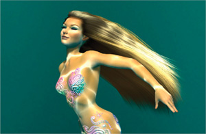
Figure 23-1 The Nalu Character
In the backstage of Nalu's hair shading, there is a system that generates the hair geometry and controls the dynamics and collisions at every frame. It is basically split in two parts: the geometry generation and the dynamics/collision computations.
The hair is made of 4,095 individual hairs that are rendered using line primitives. We used 123,000 vertices just for the hair rendering. Sending all those vertices through the dynamics and collision detection would be prohibitively slow, so we use control hairs: Nalu's haircut can be described and controlled by a smaller set of hundreds of hairs, even though the rendering requires thousands. All the expensive dynamics computations are applied only to these control hairs.
We had no time and no tools to animate the control hair structure by hand. Even if we had had the tools, hand animating so many control hairs is very difficult. A lot of subtle secondary motion is needed to make the hair look believable. See Figure 23-2. Physically based animation helped a lot.
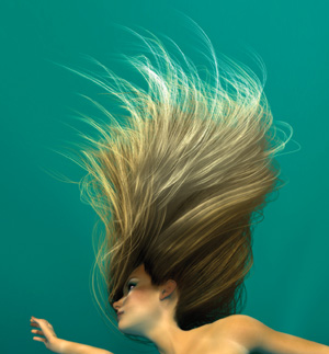
Figure 23-2 Nalu's Hair
Of course, when procedural animation is introduced, some control over the hair motion is lost (in our case, that meant losing 90 percent of the control). Collision detection and response can introduce undesired hair behavior that gets in the way of a creative animation. Our animators did a great job of understanding the inner workings of the dynamics and created some workarounds. A few additional tools were added on the engineering side to get that remaining 10 percent of human control over the dynamics.
23.1 Hair Geometry
23.1.1 Layout and Growth
The control hair structure is used to roughly describe the haircut. We "grow" the control hairs from a dedicated geometry built in Maya that represents the "scalp" (which is invisible at render time). A control hair grows from each vertex of the scalp, along the normal, as shown in Figure 23-3. The growth is 100 percent procedural.
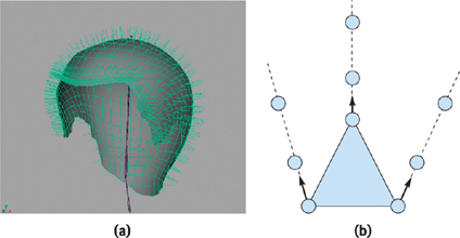
Figure 23-3 Growing Hair
23.1.2 Controlling the Hair
Once we have a set of control hairs, we subject them to physics, dynamics, and collision computations, in order to procedurally animate the hair. In this demo, the motion relies almost entirely on the dynamics. Though such a system may seem attractive, it is much more desirable to have a human-controllable system. When we want to dramatize the animation, we need to be able to "fake" or "fix" the hair behaviors. Additionally, our hair dynamics are not realistic enough to move like real hair in some situations. Having better manual control would allow us to make the motion even more convincing.
23.1.3 Data Flow
Because the hair is totally dynamic and changes every frame, we need to rebuild the final rendering hair set every frame. Figure 23-4 shows how the data moves through the process. The animated control hairs are converted to Bezier curves and tessellated to get smooth lines. The smoothed lines are then interpolated to increase the hair density. The set of interpolated hair is sent to the engine for final frame rendering. We use a dynamic vertex buffer to hold the vertex data.
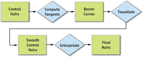
Figure 23-4 How Data Flows When Constructing the Hair
23.1.4 Tessellation
The hair tessellation process consists of smoothing each control hair by adding vertices. We increase more than fivefold, from 7 to 36 vertices. See Figures 23-5 and 23-6.
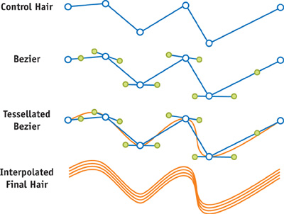
Figure 23-5 Visualizing the Steps in Creating Nalu's Hair
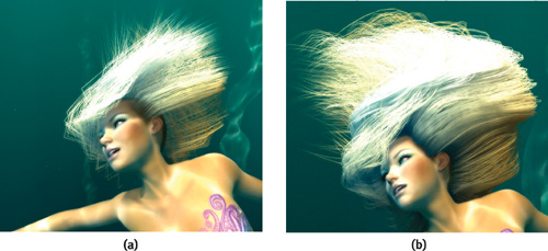
Figure 23-6 The Effect of Tessellation and Interpolation
To compute the new vertices' positions, we convert the control hairs to Bezier curves by calculating their tangents (for every frame) and using them to compute the Bezier control points. From the Bezier curves, we compute the positions of extra vertices introduced to smooth the control hairs.
The smoothed control hairs will be replicated by interpolation to create a dense set of hair, ready for final rendering.
23.1.5 Interpolation
The interpolated hair is created using the scalp mesh topology. See Figure 23-7. The extremities of each triangle have three smoothed control hairs (shown in green). We want to fill up the inside of the triangle surface with hairs, so we interpolate the coordinates of the control hair triplet to create new smoothed hair (shown in gray). The smooth control hairs and the smooth interpolated hairs have the same number of vertices.
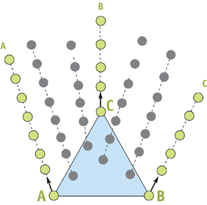
Figure 23-7 Creating the Interpolated Hair
To fill up each triangle with hairs, we use barycentric coordinates to create new, interpolated, hairs. For example, the interpolated hair Y (in Figure 23-7) is computed based on three barycentric coefficients (b A , bB , bC ), where bA + b B + b C = 1:
|
Y = A x bA + B x bB + C x bC . |
By generating two random values in [0..1], computing 1 minus the larger of them if their sum is greater than 1, and setting the third as 1 minus the other two so that they sum to 1, we can determine positions at which to grow the desired density of hair.
23.2 Dynamics and Collisions
Nalu's hair dynamics are based on a particle system, as shown in Figure 23-3b. Each uninterpolated control hair vertex is animated as a particle. The particles are not evenly spaced along a hair. The segments in a control hair are grown larger as we get away from the skull. This allows having longer hair, without adding too many vertices.
For this project, we chose to use Verlet integration to compute the particles' motion, because it tends to be more stable than Euler integration and is much simpler than Runge-Kutta integration. The explanation is beyond the scope of this chapter, but if you want to learn more about ways to use Verlet integration in games, see Jakobsen 2003.
23.2.1 Constraints
While the particles are moving around, the length of the control hairs must stay constant to avoid stretching. To make this happen, we used constraints between particles within a control hair. The constraints make the particles repel if they are too close to each other, or they contract the segment if the particles are too far apart. Of course, when we pull one particle, the length of the neighboring segment becomes invalid, so the modifications need to be applied iteratively. After several iterations, the system converges toward the desired result. See Figure 23-8.
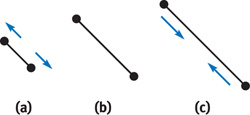
Figure 23-8 How Constraints Work to Make the Length of Hairs Stay Constant
23.2.2 Collisions
We tried many collision-detection techniques. We needed to keep the process simple and fast. For this demo, a rig of spheres turned out to work well, and it was the easiest to implement. See Figure 23-9.
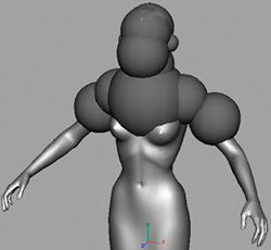
Figure 23-9 Collision Detection with Spheres
At first, the solution did not work as planned, because some hair segments were larger than the collision spheres. Because we are colliding "a point against spheres," nothing prevents the two extremities of a hair from intersecting a sphere.
To prevent this from happening, we introduced a "pearl configuration" in the control hair collision data, as shown in Figure 23-10. Instead of colliding with a point, each sphere would collide with another sphere localized on a particle.
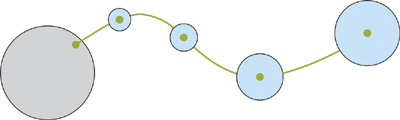
Figure 23-10 Using Pearls to Detect Collisions More Efficiently
We also tried to detect collisions between the segments and the spheres. It's not very difficult, but it's not as fast as using the "pearls." Our edge-collision detection worked reasonably well, but it had stability issues, probably due to our collision-reaction code. Regardless, we had something that worked well enough for our purposes.
23.2.3 Fins
The original conception of the mermaid included fins that were long and soft, and we considered this feature a critical part of the character. Solid fins were built and skinned to the skeleton. However, during the animation process, in Maya, the fins just followed the body, looking quite stiff. You can see what we mean in Figure 23-11.
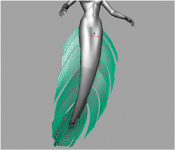
Figure 23-11 Rigid Fins on Nalu
Fortunately, our hair dynamics code can also be used to perform cloth simulation. So in the real-time engine, we compute a cloth simulation and blend the results of the cloth to the skinned geometry. A weight map was painted to define how much physics to blend in. The more we applied the physics, the softer the fins looked. On the contrary, blending more skinning resulted in a more rigid motion. We wanted the base of the fins to be more rigid than the tip, and the weight map allowed us to do exactly that, because we could paint exactly the ratio of physics versus skinning we wanted for each cloth vertex. See Figure 23-12. In the end, this combination allowed us to produce soft and realistic fins, as shown in Figure 23-13.
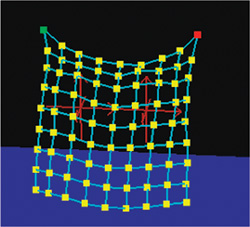
Figure 23-12 A Simple Cloth Simulation
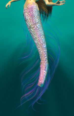
Figure 23-13 Fins in the Final Demo
23.3 Hair Shading
The problem of shading hair can be divided into two parts: a local reflectance model for hair and a method for computing self-shadowing between hairs.
23.3.1 A Real-Time Reflectance Model for Hair
For our local reflectance model, we chose the model presented in Marschner et al. 2003. We chose this model because it is a comprehensive, physically based representation of hair reflectance.
The Marschner reflectance model can be formulated as a four-dimensional bidirectional scattering function:
|
S( i , i ; o , o ), |
where i  [– /2, /2] and i [0, 2] are the input direction in polar coordinates, and o [– /2, /2] and o [0, 2] are the polar coordinates of the light direction. [1] The function S is a complete description of how a hair fiber scatters and reflects light; if we can evaluate this function, then we can compute the shading of the surface for any light position.
Because S is expensive to evaluate, we want to avoid computing it at each pixel. One possible solution is to store S in a lookup table and to read from it at runtime. This lookup table can then be encoded in a texture, allowing us to access it from a pixel shader.
Unfortunately, the function S has four parameters, and GPUs do not have native support for four-dimensional textures. This means that we would require some kind of scheme to encode a four-dimensional function in two-dimensional textures. Fortunately, if we perform our table lookups carefully, we can use only a small number of two-dimensional maps to encode the full four-dimensional function.
The Marschner Reflectance Model
The Marschner model treats each individual hair fiber as a translucent cylinder and considers the possible paths that light may take through the hair. Three types of paths are considered, each labeled differently in path notation. Path notation represents each path of light as a string of characters, each one representing a type of interaction between the light ray and a surface. R paths represent light that bounces off of the surface of the hair fiber toward the viewer. TT paths represent light that refracts into the hair and refracts out again toward the viewer. TRT paths represent light that refracts into the hair fiber, reflects off of the inside surface, and refracts out again toward the viewer. In each case, "R" represents the light reflecting, and "T" represents a ray being transmitted (or refracting) through a surface.
Marschner et al. (2003) showed that each of these paths contributes to a distinct and visually significant aspect of hair reflectance, allowing a degree of realism not possible with previous hair reflectance models. Figure 23-14 shows the three reflectance paths that contribute the most to the appearance of hair.
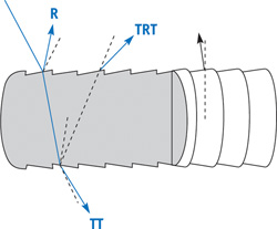
Figure 23-14 Reflectance Paths
We can thus write the reflectance model as follows:
|
S = SR + STT + STRT . |
Each term SP can be further factored as the product of two functions. The function MP describes the effect of the angles on the reflectance. The other function, NP , captures the reflection in the direction. If we assume a perfectly circular hair fiber, then we can write both M and N in terms of a smaller set of angles. By defining secondary angles d = ½( i – o ) and d = i – o , each term of the preceding equation can be written as:
|
Sp = Mp ( i , o ) x Np ( d , d ) for P = R, TT, TRT. |
In this form, we can see that both M and N are functions of only two parameters. This means that we can compute a lookup table for each of these functions and encode them in two-dimensional textures. Two-dimensional textures are ideal, because the GPU is optimized for two-dimensional texturing. We can also use the GPU's interpolation and mipmapping functionality to eliminate shader aliasing. [2]
Although we are storing six functions, many of them are only single channel and can be stored in the same texture. M R , MTT , and MTRT are each only a single channel, and so they are packed together into the first lookup texture. NR is a single channel, but NTT and NTRT are each three channels. We store NTT and NR together in the second lookup texture. To improve performance and reduce texture usage in the demo, we made a simplifying assumption that M TT ( i , o ) = M TRT ( i , o ). This allowed us to store NTT and NTRT in the same texture, and to cut the number of textures from three down to two. See Figures 23-15 and 23-16.
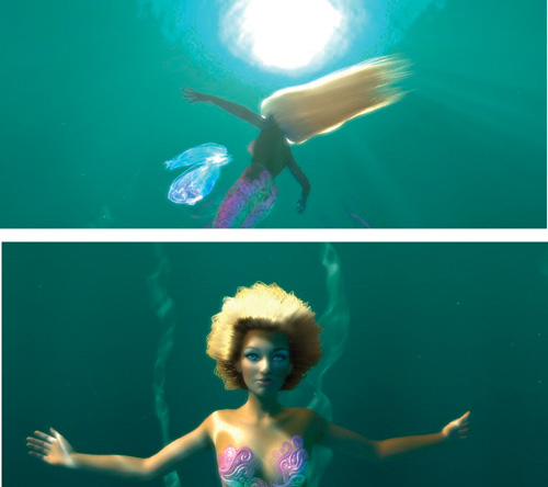
Figure 23-15 Reflectance
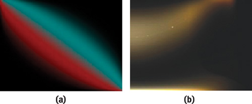
Figure 23-16 Lookup Textures for the Marschner Hair Reflectance Model
Although the model is expressed in terms of angles, computing these angles from vectors would require inverse trigonometric functions. These are expensive, and we would like to avoid them if possible. Instead of passing down i and o into the first lookup, we compute the sines:
|
sin i = (light · Tangent), |
|
sin o = (eye · Tangent). |
We can then express M as a function of sin i and sin o , saving some math in the shader.
With a little more work, we can also compute cos d . We first project the eye and light vectors perpendicular to the hair as follows:
|
lightPerp = light – (light · tangent) x tangent, |
|
eyePerp = eye – (eye · tangent) x tangent. |
Then from the formula
|
(lightPerp · eyePerp) = ||lightPerp|| x ||eyePerp|| x cos d , |
we can compute cos d as follows:
|
cos d |
= |
(eyePerp · lightPerp) x |
|
((eyePerp · eyePerp) x (lightPerp · lightPerp))-0.5. |
The only angle left to calculate is d . To do so, we note that d is a function of i and o . Because we are already using a lookup table indexed by i and o , we can add an extra channel to the lookup table that stores d .
Listing 23-1 is a brief summary of our shader in pseudocode.
In our implementation, the lookup tables were computed on the CPU. We used 128 x 128 textures with an 8-bit-per-component format. The 8-bit format required us to scale the values to be in the range [0..1]. As a result, we had to add an extra scale factor in the shader to balance out the relative intensities of the terms. If more accuracy were desired, we could skip this step and use 16-bit floating-point textures to store the lookup tables. We found this unnecessary for our purposes.
To actually compute one of these lookup tables, we had to write a program to evaluate the functions M and N. These functions are too complicated to present here; Marschner et al. 2003 provides a complete description as well as a derivation.
Example 23-1. Pseudocode Summarizing the Shaders
// In the Vertex Shader:
SinThetaI = dot(light, tangent) SinThetaO = dot(eye, tangent) LightPerp =
    light –– SinThetaI *tangent eyePerp = eye – SinThetaO * tangent;
CosPhiD = dot(eyePerp, lightPerp) *
              (dot(eyePerp, eyePerp) * dot(lightPerp, lightPerp)) ^
          -0.5
          // In the Fragment Shader:
          (MR, MTT, MTRT, cosThetaD) = lookup1(cosThetaI, cosThetaO)(NTT, NR) =
              lookup2(CosPhiD, cosThetaD) NTRT = lookup3(CosPhiD, cosThetaD) S =
                  MR * NR + MTT * NTT + MTRT * NTRT
Note that there are many other parameters to the reflectance model that are encoded in the lookup tables. These include the width and strength of highlights and the color and index of refraction of the hair, among others. In our implementation, we allowed these parameters to be altered at runtime, and we recomputed the lookup tables on the fly.
Solid Geometry
Though we used this hair reflectance model for rendering hair represented as line strips, it is possible to extend it to hair that is represented as solid geometry. Instead of using the tangent of a line strip, we could use one of the primary tangents of the surface. Finally, we must take into account self-occlusion by the surface. This is done by multiplying by an extra term (wrap + dot(N, L)) / (1 + wrap) where dot(N, L) is the dot product between the normal light vector and wrap is a value between zero and one that controls how far the lighting is allowed to wrap around the model. This is a simple approximation used to simulate light bleeding through the hair (Green 2004).
23.3.2 Real-Time Volumetric Shadows in Hair
Shadows in real-time applications are usually computed with one of two methods: stencil shadow volumes or shadow maps. Unfortunately, neither of these techniques works well for computing shadows on hair. The sheer amount of geometry used in the hair would make stencil shadow volumes intractable, and shadow maps exhibit severe aliasing on highly detailed geometry such as hair.
Instead, we used an approach to shadow rendering specifically designed for rendering shadows in hair. Opacity shadow maps extend shadow mapping to handle volumetric objects and antialiasing (Kim and Neumann 2001). Opacity shadow maps were originally implemented on GeForce 2-class hardware, where the flexibility in terms of programmability was much more limited than what is available on current GPUs. The original implementation did not achieve real-time performance on large data sets, and it required a large portion of the algorithm to be run on the CPU. GeForce 6 Series hardware has sufficient programmability that we can execute the majority of the algorithm on the GPU. In doing so, we achieve real-time performance even for a large hair data set.
Opacity Shadow Maps
Rather than use a discrete test such as traditional shadow maps, we use opacity shadow maps, which allow fractional shadow values. This means that rather than a simple binary test for occlusion, we need a measure of the percentage of light that penetrates to depth z (in light space) over a given pixel. This is given by the following formula:
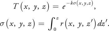
T(x, y, z) is the fraction of light penetrating to depth z at pixel location (x, y), is called the opacity thickness, and r(x, y, z) is the extinction coefficient, which describes the percentage of light that is absorbed per unit distance at the point (x, y, z). The value k is a constant chosen such that when = 1, T is approximately 0 (within numerical precision). This allows us to ignore values outside of the range [0..1].
The idea of opacity shadow maps is to compute at a discrete set of z values z 0. . . z n-1. Then we determine in-between values for by interpolation between the two nearest values as follows:
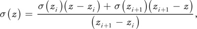
where z i < z < z i+1.
This is a reasonable approximation, because sigma is a strictly increasing function of z. We take n to be 16, with z 0 being the near plane of the hair in light space, and z 15 being the far plane of the hair in light space. The other planes were distributed uniformly apart, so that z i = z 0 + i dz, where dz = (z 15 – z 0)/16. Note that because r is 0 outside of the hair volume, (x, y, z 0) = 0 for all x and y, and so we only have to store at z = z 1. . . z 15.
Kim and Neumann (2001) noted that the integral sigma could be computed using additive blending on graphics hardware. Our implementation also uses hardware blending, but it also uses shaders to reduce the amount of work done by the CPU.
An Updated Implementation
The naive approach would be to store (x, y, z i ) in 16 textures. This would require that we render 16 times to generate the full opacity shadow map. Our first observation is that storing requires only 1 channel, so we can pack up to 4 sigma values into a single 4-channel texture and render to all of them simultaneously. Using this scheme, we can reduce the number of render passes from 16 to 4.
We can do better than 4 render passes, however, if we use multiple render targets (MRT). MRT is a feature that allows us to render to up to 4 different textures simultaneously. If we use MRT, we can render to 4 separate 4-channel textures simultaneously, allowing us to render to all 16 channels in just a single render pass.
Now if we simply blend additively to every channel, then we will get every strand of hair contributing to every layer. What we really want is for each layer i to be affected by only those parts of the hair with z hair < z i . With a shader, we can simply output 0 if zhair > z i .
Performing a Lookup
Given an opacity shadow map, we must evaluate T at the point (x, y, z), given the slices of the opacity shadow map. We do this by linearly interpolating the values of sigma from the two nearest slices. The value at (x, y, z) is a linear combination of (x, y, z 0)... (x, y, zn ). In particular,
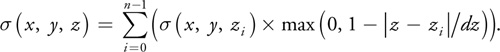
We can compute wi = |z – z i |/dz in the vertex shader for all 16 values.
// depth1 contains z0..z3, inverseDeltaD = 1/dz.
v2f.OSM1weight = max(0.0.xxxx, 1 - abs(dist - depth1) * inverseDeltaD);
v2f.OSM2weight = max(0.0.xxxx, 1 - abs(dist - depth2) * inverseDeltaD);
v2f.OSM3weight = max(0.0.xxxx, 1 - abs(dist - depth3) * inverseDeltaD);
v2f.OSM4weight = max(0.0.xxxx, 1 - abs(dist - depth4) * inverseDeltaD);
To improve performance, we compute these weights in the vertex shader and pass them directly to the fragment shader. Although the results are not mathematically equivalent to computing the weights in the fragment shader, they are close enough for our purposes.
Once these weights have been computed, it is simply a matter of computing the sum
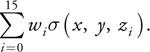
Because of the way the data is aligned, we can compute
in a single dot product, and we can compute the sums for i = 4..7, i = 8..11, and i = 12..15 with dot products similarly.
/* Compute the total density */
half density = 0;
density = dot(h4tex2D(OSM1, v2f.shadowCoord.xy), v2f.OSM1weight);
density += dot(h4tex2D(OSM2, v2f.shadowCoord.xy), v2f.OSM2weight);
density += dot(h4tex2D(OSM3, v2f.shadowCoord.xy), v2f.OSM3weight);
density += dot(h4tex2D(OSM4, v2f.shadowCoord.xy), v2f.OSM4weight);
Finally, we compute transmittance from optical density to get a value between 0 and 1 that represents the fraction of light that reaches the point (x, y, z) from the light source. We multiply this value by the shading value to get the final color of the hair.
half shadow = exp(-5.5 * density);Figure 23-17 shows the dramatic difference between shadowed and unshadowed hair.
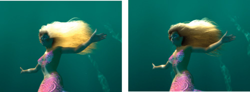
Figure 23-17 Comparing Shadowed and Unshadowed Hair
23.4 Conclusion and Future Work
We have shown that it is now possible to simulate all aspects of hair rendering in real time: from animation and dynamics to rendering and shading. We hope that our system will provide a basis for real-time rendering of hair in interactive applications such as games.
Although the ideas here have been applied to the animation and rendering of hair, this is not their only application. The Marschner reflectance model has a natural factorization that we used to decompose it into texture lookups. This approach can be extended to any reflectance model by using approximate factorizations (McCool et al. 2001). These numerical factorizations have all the advantages of analytical factorizations, with the exception of a small amount of error.
Opacity shadow maps, in addition to being extremely useful for rendering hair, can also be used for cases where depth maps fail. For example, they could be applied to volumetric representations such as clouds and smoke, or to highly detailed objects such as dense foliage.
As GPUs become more flexible, it is worthwhile to look for ways to transfer more work to them. This includes not only obviously parallel tasks such as tessellation and interpolation, but also domains more traditionally given to CPUs, such as collision detection and physics.
Performance is not our only focus; we are also looking at making the hair more controllable by the developers, so that it becomes easy to style and animate. Many challenges are ahead, but we hope to see more realistic hair in next-generation applications.
23.5 References
Green, Simon. 2004. "Real-Time Approximations to Subsurface Scattering." In GPU Gems, edited by Randima Fernando, pp. 263–278. Addison-Wesley.
Jakobsen, Thomas. 2003. "Advanced Character Physics." IO Interactive.
Kim, T.-Y., and U. Neumann. 2001. "Opacity Shadow Maps." In Proceedings of SIGGRAPH 2001, pp. 177–182.
Marschner, S. R., H. W. Jensen, M. Cammarano, S. Worley, and P. Hanrahan. 2003. "Light Scattering from Human Hair Fibers." ACM Transactions on Graphics (Proceedings of SIGGRAPH 2003) 22(3), pp. 780–791.
McCool, Michael D., Jason Ang, and Anis Ahmad. 2001. "Homomorphic Factorizations of BRDFs for High-Performance Rendering." In Proceedings of SIGGRAPH 2001, pp. 171–178.
Copyright
Many of the designations used by manufacturers and sellers to distinguish their products are claimed as trademarks. Where those designations appear in this book, and Addison-Wesley was aware of a trademark claim, the designations have been printed with initial capital letters or in all capitals.
The authors and publisher have taken care in the preparation of this book, but make no expressed or implied warranty of any kind and assume no responsibility for errors or omissions. No liability is assumed for incidental or consequential damages in connection with or arising out of the use of the information or programs contained herein.
NVIDIA makes no warranty or representation that the techniques described herein are free from any Intellectual Property claims. The reader assumes all risk of any such claims based on his or her use of these techniques.
The publisher offers excellent discounts on this book when ordered in quantity for bulk purchases or special sales, which may include electronic versions and/or custom covers and content particular to your business, training goals, marketing focus, and branding interests. For more information, please contact:
U.S. Corporate and Government Sales
(800) 382-3419
corpsales@pearsontechgroup.com
For sales outside of the U.S., please contact:
International Sales
international@pearsoned.com
Visit Addison-Wesley on the Web: www.awprofessional.com
Library of Congress Cataloging-in-Publication Data
GPU gems 2 : programming techniques for high-performance graphics and general-purpose
computation / edited by Matt Pharr ; Randima Fernando, series editor.
p. cm.
Includes bibliographical references and index.
ISBN 0-321-33559-7 (hardcover : alk. paper)
1. Computer graphics. 2. Real-time programming. I. Pharr, Matt. II. Fernando, Randima.
T385.G688 2005
006.66—dc22
2004030181
GeForce™ and NVIDIA Quadro® are trademarks or registered trademarks of NVIDIA Corporation.
Nalu, Timbury, and Clear Sailing images © 2004 NVIDIA Corporation.
mental images and mental ray are trademarks or registered trademarks of mental images, GmbH.
Copyright © 2005 by NVIDIA Corporation.
All rights reserved. No part of this publication may be reproduced, stored in a retrieval system, or transmitted, in any form, or by any means, electronic, mechanical, photocopying, recording, or otherwise, without the prior consent of the publisher. Printed in the United States of America. Published simultaneously in Canada.
For information on obtaining permission for use of material from this work, please submit a written request to:
Pearson Education, Inc.
Rights and Contracts Department
One Lake Street
Upper Saddle River, NJ 07458
Text printed in the United States on recycled paper at Quebecor World Taunton in Taunton, Massachusetts.
Second printing, April 2005
Dedication
To everyone striving to make today's best computer graphics look primitive tomorrow
- Copyright
- Inside Back Cover
- Inside Front Cover
- Part I: Geometric Complexity
-
- Chapter 1. Toward Photorealism in Virtual Botany
- Chapter 2. Terrain Rendering Using GPU-Based Geometry Clipmaps
- Chapter 3. Inside Geometry Instancing
- Chapter 4. Segment Buffering
- Chapter 5. Optimizing Resource Management with Multistreaming
- Chapter 6. Hardware Occlusion Queries Made Useful
- Chapter 7. Adaptive Tessellation of Subdivision Surfaces with Displacement Mapping
- Chapter 8. Per-Pixel Displacement Mapping with Distance Functions
- Part II: Shading, Lighting, and Shadows
-
- Chapter 9. Deferred Shading in S.T.A.L.K.E.R.
- Chapter 10. Real-Time Computation of Dynamic Irradiance Environment Maps
- Chapter 11. Approximate Bidirectional Texture Functions
- Chapter 12. Tile-Based Texture Mapping
- Chapter 13. Implementing the mental images Phenomena Renderer on the GPU
- Chapter 14. Dynamic Ambient Occlusion and Indirect Lighting
- Chapter 15. Blueprint Rendering and "Sketchy Drawings"
- Chapter 16. Accurate Atmospheric Scattering
- Chapter 17. Efficient Soft-Edged Shadows Using Pixel Shader Branching
- Chapter 18. Using Vertex Texture Displacement for Realistic Water Rendering
- Chapter 19. Generic Refraction Simulation
- Part III: High-Quality Rendering
-
- Chapter 20. Fast Third-Order Texture Filtering
- Chapter 21. High-Quality Antialiased Rasterization
- Chapter 22. Fast Prefiltered Lines
- Chapter 23. Hair Animation and Rendering in the Nalu Demo
- Chapter 24. Using Lookup Tables to Accelerate Color Transformations
- Chapter 25. GPU Image Processing in Apple's Motion
- Chapter 26. Implementing Improved Perlin Noise
- Chapter 27. Advanced High-Quality Filtering
- Chapter 28. Mipmap-Level Measurement
- Part IV: General-Purpose Computation on GPUS: A Primer
-
- Chapter 29. Streaming Architectures and Technology Trends
- Chapter 30. The GeForce 6 Series GPU Architecture
- Chapter 31. Mapping Computational Concepts to GPUs
- Chapter 32. Taking the Plunge into GPU Computing
- Chapter 33. Implementing Efficient Parallel Data Structures on GPUs
- Chapter 34. GPU Flow-Control Idioms
- Chapter 35. GPU Program Optimization
- Chapter 36. Stream Reduction Operations for GPGPU Applications
- Part V: Image-Oriented Computing
-
- Chapter 37. Octree Textures on the GPU
- Chapter 38. High-Quality Global Illumination Rendering Using Rasterization
- Chapter 39. Global Illumination Using Progressive Refinement Radiosity
- Chapter 40. Computer Vision on the GPU
- Chapter 41. Deferred Filtering: Rendering from Difficult Data Formats
- Chapter 42. Conservative Rasterization
- Part VI: Simulation and Numerical Algorithms
-
- Chapter 43. GPU Computing for Protein Structure Prediction
- Chapter 44. A GPU Framework for Solving Systems of Linear Equations
- Chapter 45. Options Pricing on the GPU
- Chapter 46. Improved GPU Sorting
- Chapter 47. Flow Simulation with Complex Boundaries
- Chapter 48. Medical Image Reconstruction with the FFT