
GPU Gems 2
GPU Gems 2 is now available, right here, online. You can purchase a beautifully printed version of this book, and others in the series, at a 30% discount courtesy of InformIT and Addison-Wesley.
The CD content, including demos and content, is available on the web and for download.
Chapter 37. Octree Textures on the GPU
Sylvain Lefebvre
GRAVIR/IMAG – INRIA
Samuel Hornus
GRAVIR/IMAG – INRIA
Fabrice Neyret
GRAVIR/IMAG – INRIA
Texture mapping is a very effective and efficient technique for enriching the appearance of polygonal models with details. Textures store not only color information, but also normals for bump mapping and various shading attributes to create appealing surface effects. However, texture mapping usually requires parameterizing a mesh by associating a 2D texture coordinate with every mesh vertex. Distortions and seams are often introduced by this difficult process, especially on complex meshes.
The 2D parameterization can be avoided by defining the texture inside a volume enclosing the object. Debry et al. (2002) and Benson and Davis (2002) have shown how 3D hierarchical data structures, named octree textures, can be used to efficiently store color information along a mesh surface without texture coordinates. This approach has two advantages. First, color is stored only where the surface intersects the volume, thus reducing memory requirements. Figures 37-1 and 37-2 illustrate this idea. Second, the surface is regularly sampled, and the resulting texture does not suffer from any distortions. In addition to mesh painting, any application that requires storing information on a complex surface can benefit from this approach.

Figure 37-1 An Octree Texture Surrounding a 3D Model
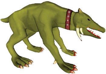
Figure 37-2 Unparameterized Mesh Textures with an Octree Texture
This chapter details how to implement octree textures on today's GPUs. The octree is directly stored in texture memory and accessed from a fragment program. We discuss the trade-offs between performance, storage efficiency, and rendering quality. After explaining our implementation in Section 37.1, we demonstrate it on two different interactive applications:
- A surface-painting application (Section 37.2). In particular, we discuss the different possibilities for filtering the resulting texture (Section 37.2.3). We also show how a texture defined in an octree can be converted into a standard texture, possibly at runtime (Section 37.2.4).
- A nonphysical simulation of liquid flowing along a surface (Section 37.3). The simulation runs entirely on the GPU.
37.1 A GPU-Accelerated Hierarchical Structure: The N3-Tree
37.1.1 Definition
An octree is a regular hierarchical data structure. The first node of the tree, the root, is a cube. Each node has either eight children or no children. The eight children form a 2x2x2 regular subdivision of the parent node. A node with children is called an internal node. A node without children is called a leaf. Figure 37-3 shows an octree surrounding a 3D model where the nodes that have the bunny's surface inside them have been refined and empty nodes have been left as leaves.
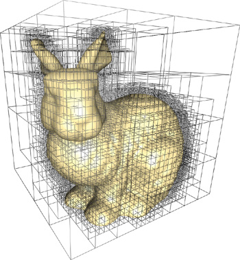
Figure 37-3 An Octree Surrounding a 3D Model
In an octree, the resolution in each dimension increases by two at each subdivision level. Thus, to reach a resolution of 256x256x256, eight levels are required (28= 256). Depending on the application, one might prefer to divide each edge by an arbitrary number N rather than 2. We therefore define a more generic structure called an N3 -tree. In an N3-tree, each node has N 3 children. The octree is an N3-tree with N = 2. A larger value of N reduces the tree depth required to reach a given resolution, but it tends to waste memory because the surface is less closely matched by the tree.
37.1.2 Implementation
To implement a hierarchical tree on a GPU, we need to define how to store the structure in texture memory and how to access the structure from a fragment program.
A simple approach to implement an octree on a CPU is to use pointers to link the tree nodes together. Each internal node contains an array of pointers to its children. A child can be another internal node or a leaf. A leaf contains only a data field.
Our implementation on the GPU follows a similar approach. Pointers simply become indices within a texture. They are encoded as RGB values. The content of the leaves is directly stored as an RGB value within the parent node's array of pointers. We use the alpha channel to distinguish between a pointer to a child and the content of a leaf. Our approach relies on dependent texture lookups (or texture indirections). This requires the hardware to support an arbitrary number of dependent texture lookups, which is the case for GeForce FX and GeForce 6 Series GPUs.
The following sections detail our GPU implementation of the N3-tree. For clarity, the figures illustrate the 2D equivalent of an octree (a quadtree).
Storage
We store the tree in an 8-bit RGBA 3D texture called the indirection pool. Each "pixel" of the indirection pool is called a cell.
The indirection pool is subdivided into indirection grids. An indirection grid is a cube of NxNxN cells (a 2x2x2 grid for an octree). Each node of the tree is represented by an indirection grid. It corresponds to the array of pointers in the CPU implementation described earlier.
A cell of an indirection grid can be empty or can contain one of the following:
- Data, if the corresponding child is a leaf
- The index of an indirection grid, if the corresponding child is another internal node
Figure 37-4 illustrates our tree storage representation.
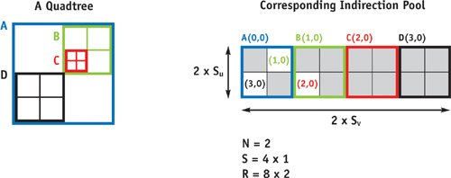
Figure 37-4 Storage in Texture Memory (2D Case)
We note S = Su x Sv x Sw as the number of indirection grids stored in the indirection pool and R= (N x Su ) x (N x Sv ) x (N x Sw ) as the resolution in cells of the indirection pool.
Data values and indices of children are both stored as RGB triples. The alpha channel is used as a flag to determine the cell content (alpha = 1 indicates data; alpha = 0.5 indicates index; alpha = 0 indicates empty cell). The root of the tree is always stored at (0, 0, 0) within the indirection pool.
Accessing the Structure: Tree Lookup
Once the tree is stored in texture memory, we need to access it from a fragment program. As with standard 3D
textures, the tree defines a texture within the unit cube. We want to retrieve the value stored in the tree at a
point M
 [0, 1]3. The tree lookup starts from the root and successively visits the nodes containing the point
M until a leaf is reached.
[0, 1]3. The tree lookup starts from the root and successively visits the nodes containing the point
M until a leaf is reached.
Let I D be the index of the indirection grid of the node visited at depth D. The tree lookup is initialized with I 0= (0, 0, 0), which corresponds to the tree root. When we are at depth D, we know the index I D of the current node's indirection grid. We now explain how we retrieve I D+1 from I D .
The lookup point M is inside the node visited at depth D. To decide what to do next, we need to read from the indirection grid ID the value stored at the location corresponding to M. To do so, we need to compute the coordinates of M within the node.
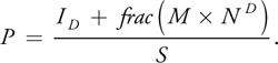
At depth D, a complete tree produces a regular grid of resolution N D x N D x N D within the unit cube. We call this grid the depth-D grid. Each node of the tree at depth D corresponds to a cell of this grid. In particular, M is within the cell corresponding to the node visited at depth D. The coordinates of M within this cell are given by frac(M x N D ). We use these coordinates to read the value from the indirection grid I D . The lookup coordinates within the indirection pool are thus computed as:
We then retrieve the RGBA value stored at P in the indirection pool. Depending on the alpha value, either we will return the RGB color if the child is a leaf, or we will interpret the RGB values as the index of the child's indirection grid (I D+1) and continue to the next tree depth. Figure 37-5 summarizes this entire process for the 2D case (quadtree).
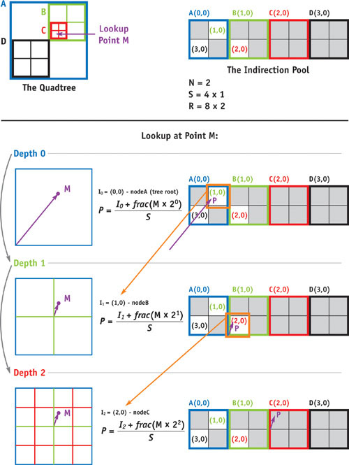
Figure 37-5 Example of a Tree Lookup
The lookup ends when a leaf is reached. In practice, our fragment program also stops after a fixed number of texture lookups: on most hardware, it is only possible to implement loop statements with a fixed number of iterations (however, early exit is possible on GeForce 6 Series GPUs). The application is in charge of limiting the tree depth with respect to the maximum number of texture lookups done within the fragment program. The complete tree lookup code is shown in Listing 37-1.
Example 37-1. The Tree Lookup Cg Code
float4 tree_lookup(uniform sampler3D IndirPool, // Indirection Pool
                   uniform float3 invS,
                   // 1 / S
                   uniform float N,
                   float3 M) // Lookup coordinates
{
  float4 I = float4(0.0, 0.0, 0.0, 0.0);
  float3 MND = M;
  for (float i = 0; i < HRDWTREE_MAX_DEPTH; i++)
  { // fixed # of iterations
    float3 P;
    // compute lookup coords. within current node
    P = (MND + floor(0.5 + I.xyz * 255.0)) * invS;
    // access indirection pool
    if (I.w < 0.9)
      // already in a leaf?
      I = (float4)tex3D(IndirPool, P); // no, continue to next depth
#ifdef DYN_BRANCHING // early exit if hardware supports dynamic branching
    if (I.w > 0.9)
      // a leaf has been reached
      break;
#endif
    if (I.w < 0.1) // empty cell
      discard;
    // compute pos within next depth grid
    MND = MND * N;
  }
  return (I);
}
Further Optimizations
In our tree lookup algorithm, as we explained earlier, the computation of P requires a frac instruction. In our implementation, however, as shown Listing 37-1, we actually avoid computing the frac by relying on the cyclic behavior of the texture units (repeat mode). We leave the detailed explanations as an appendix, located on the book's CD.
We compute P as
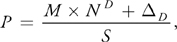
where D is an integer within the range [0, S[.
We store D instead of directly storing the I D values. Please refer to the appendix on the CD for the code to compute D .
Encoding Indices
The indirection pool is an 8-bit 3D RGBA texture. This means that we can encode only 256 different values per channel. This gives us an addressing space of 24 bits (3 indices of 8 bits), which makes it possible to encode octrees large enough for most applications.
Within a fragment program, a texture lookup into an 8-bit texture returns a value mapped between [0,1]. However, we need to encode integers. Using a floating-point texture to do so would require more memory and would reduce performance. Instead, we map values between [0,1] with a fixed precision of 1/255 and simply multiply the floating-point value by 255 to obtain an integer. Note that on hardware without fixed-precision registers, we need to compute floor(0.5 + 255 * v) to avoid rounding errors.
37.2 Application 1: Painting on Meshes
In this section we use the GPU-accelerated octree structure presented in the previous section to create a surface-painting application. Thanks to the octree, the mesh does not need to be parameterized. This is especially useful with complex meshes such as trees, hairy monsters, or characters.
The user will be able to paint on the mesh using a 3D brush, similar to the brush used in 2D painting applications. In this example, the painting resolution is homogeneous along the surface, although multiresolution painting would be an easy extension if desired.
37.2.1 Creating the Octree
We start by computing the bounding box of the object to be painted. The object is then rescaled such that its largest dimension is mapped between [0,1]. The same scaling is applied to the three dimensions because we want the painting resolution to be the same in every dimension. After this process, the mesh fits entirely within the unit box.
The user specifies the desired resolution of the painting. This determines the depth of the leaves of the octree that contain colors. For instance, if the user selects a resolution of 5123, the leaves containing colors will be at depth 9.
The tree is created by subdividing the nodes intersecting the surface until all the leaves either are empty or are at the selected depth (color leaves). To check whether a tree node intersects the geometry, we rely on the box defining the boundary of the node. This process is depicted in Figure 37-6. We use the algorithm shown in Listing 37-2.
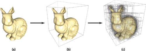
Figure 37-6 Building an Octree Around a Mesh Surface
This algorithm uses our GPU octree texture API. The links between nodes (indices in the indirection grids) are set up by the createChild() call. The values stored in tree leaves are set up by calling setChildAsEmpty() and setChildColor(), which also set the appropriate alpha value.
Example 37-2. Recursive Algorithm for Octree Creation
 void createNode(depth, polygons, box)
for all children (i, j, k) within (N, N, N)
if (depth + 1 == painting depth)
// painting depth reached?
setChildColor(i, j, k, white)
// child is at depth+1
else
childbox = computeSubBox(i, j, k, box)
if (childbox intersect polygons)
child = createChild(i, j, k)
// recurse
createNode(depth + 1, polygons, childbox)
else
setChildAsEmpty(i, j, k)
37.2.2 Painting
In our application, the painting tool is drawn as a small sphere moving along the surface of the mesh. This sphere is defined by a painting center P center and a painting radius P radius. The behavior of the brush is similar to that of brushes in 2D painting tools.
When the user paints, the leaf nodes intersecting the painting tool are updated. The new color is computed as a weighted sum of the previous color and the painting color. The weight is such that the painting opacity decreases as the distance from P center increases.
To minimize the amount of data to be sent to the GPU as painting occurs, only the modified leaves are updated in texture memory. This corresponds to a partial update of the indirection pool texture (under OpenGL, we use glTexSubImage3D). The modifications are tracked on a copy of the tree stored in CPU memory.
37.2.3 Rendering
To render the textured mesh, we need to access the octree from the fragment program, using the tree lookup defined in Section 37.1.2.
The untransformed coordinates of the vertices are stored as 3D texture coordinates. These 3D texture coordinates are interpolated during the rasterization of the triangles. Therefore, within the fragment program, we know the 3D point of the mesh surface being projected in the fragment. By using these coordinates as texture coordinates for the tree lookup, we retrieve the color stored in the octree texture.
However, this produces the equivalent of a standard texture lookup in "nearest" mode. Linear interpolation and mipmapping are often mandatory for high-quality results. In the following section, we discuss how to implement these techniques for octree textures.
Linear Interpolation
Linear interpolation of the texture can be obtained by extending the standard 2D linear interpolation. Because the octree texture is a volume texture, eight samples are required for linear interpolation, as shown in Figure 37-7.
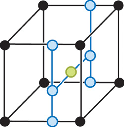
Figure 37-7 Linear Interpolation Using Eight Samples
However, we store information only where the surface intersects the volume. Some of the samples involved in the 3D linear interpolation are not on the surface and have no associated color information. Consider a sample at coordinates (i, j, k) within the maximum depth grid (recall that the depth D grid is the regular grid produced by a complete octree at depth D). The seven other samples involved in the 3D linear interpolation are at coordinates (i+1, j, k), (i, j+1, k), (i, j, k+1), (i, j+1, k+1), (i+1, j, k+1), (i+1, j+1, k), and (i+1, j+1, k+1). However, some of these samples may not be included in the tree, because they are too far from the surface. This leads to rendering artifacts, as shown in Figure 37-8.
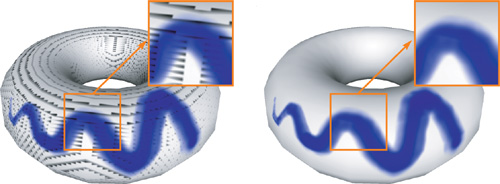
Figure 37-8 Fixing Artifacts Caused by Straightforward Linear Interpolation
We remove these artifacts by modifying the tree creation process. We make sure that all of the samples necessary for linear interpolation are included in the tree. This can be done easily by enlarging the box used to check whether a tree node intersects the geometry. The box is built in such a way that it includes the previous samples in each dimension. Indeed, the sample at (i, j, k) must be added if one of the previous samples (for example, the one at (i-1, j-1, k-1)) is in the tree. This is illustrated in Figure 37-9.
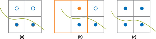
Figure 37-9 Modifying the Tree Creation to Remove Linear Interpolation Artifacts
In our demo, we use the same depth for all color leaves. Of course, the octree structure makes it possible to store color information at different depths. However, doing so complicates linear interpolation. For more details, refer to Benson and Davis 2002.
Mipmapping
When a textured mesh becomes small on the screen, multiple samples of the texture fall into the same pixel. Without a proper filtering algorithm, this leads to aliasing. Most GPUs implement the mipmapping algorithm on standard 2D textures. We extend this algorithm to our GPU octree textures.
We define the mipmap levels as follows. The finest level (level 0) corresponds to the leaves of the initial octree. A coarser level is built from the previous one by merging the leaves in their parent node. The node color is set to the average color of its leaves, and the leaves are suppressed, as shown in Figure 37-10. The octree depth is therefore reduced by one at each mipmapping level. The coarsest level has only one root node, containing the average color of all the leaves of the initial tree.
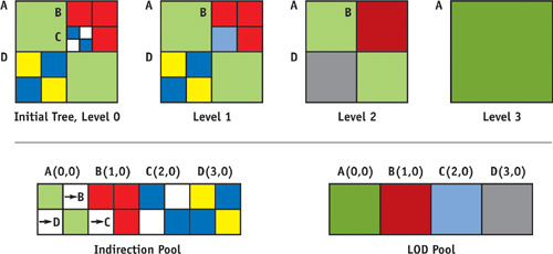
Figure 37-10 An Example of a Tree with Mipmapping
Storing one tree per mipmapping level would be expensive. Instead, we create a second 3D texture, called the LOD pool. The LOD pool has one cell per indirection grid of the indirection pool (see Figure 37-10, bottom row). Its resolution is thus S u x S v x S w (see "Storage" in Section 37.1.2). Each node of the initial tree becomes a leaf at a given mipmapping level. The LOD pool stores the color taken by the nodes when they are used as leaves in a mipmapping level.
To texture the mesh at a specific mipmapping level, we stop the tree lookup at the corresponding depth and look up the node's average color in the LOD pool. The appropriate mipmapping level can be computed within the fragment program using partial-derivative instructions.
37.2.4 Converting the Octree Texture to a Standard 2D Texture
Our ultimate goal is to use octree textures as a replacement for 2D textures, thus completely removing the need for a 2D parameterization. However, the octree texture requires explicit programming of the texture filtering. This leads to long fragment programs. On recent GPUs, performance is still high enough for texture-authoring applications, where a single object is displayed. But for applications displaying complex scenes, such as games or simulators, rendering performance may be too low. Moreover, GPUs are extremely efficient at displaying filtered standard 2D texture maps.
Being able to convert an octree texture into a standard 2D texture is therefore important. We would like to perform this conversion dynamically: this makes it possible to select the best representation at runtime. For example, an object near the viewpoint would use the linearly interpolated octree texture and switch to the corresponding filtered standard 2D texture when it moves farther away. The advantage is that filtering of the 2D texture is natively handled by the GPU. Thus, the extra cost of the octree texture is incurred only when details are visible.
In the following discussion, we assume that the mesh is already parameterized. We describe how we create a 2D texture map from an octree texture.
To produce the 2D texture map, we render the triangles using their 2D (u, v) coordinates instead of their 3D (x, y, z) coordinates. The triangles are textured with the octree texture, using the 3D coordinates of the mesh vertices as texture coordinates for the tree lookup. The result is shown in Figure 37-11.
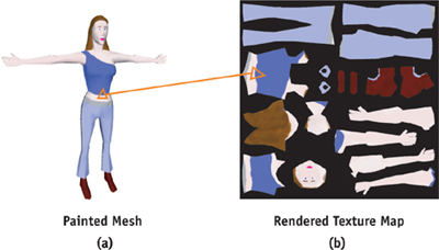
Figure 37-11 Converting the Octree into a Standard 2D Texture
However, this approach produces artifacts. When the 2D texture is applied to the mesh with filtering, the background color bleeds inside the texture. This happens because samples outside of the 2D triangles are used by the linear interpolation for texture filtering. It is not sufficient to add only a few border pixels: more and more pixels outside of the triangles are used by coarser mipmapping levels. These artifacts are shown in Figure 37-12.
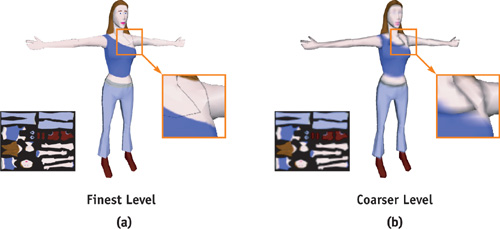
Figure 37-12 Artifacts Resulting from Straightforward Conversion
To suppress these artifacts, we compute a new texture in which the colors are extrapolated outside of the 2D triangles. To do so, we use a simplified GPU variant of the extrapolation method known as push-pull. This method has been used for the same purpose in Sander et al. 2001.
We first render the 2D texture map as described previously. The background is set with an alpha value of 0. The triangles are rendered using an alpha value of 1. We then ask the GPU to automatically generate the mipmapping levels of the texture. Then we collapse all the mipmapping levels into one texture, interpreting the alpha value as a transparency coefficient. This is done with the Cg code shown in Listing 37-3.
Finally, new mipmapping levels are generated by the GPU from this new texture. Figures 37-13 and 37-14 show the result of this process.
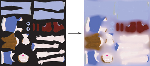
Figure 37-13 Color Extrapolation
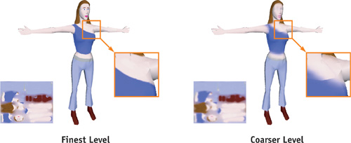
Figure 37-14 Artifacts Removed Due to Color Extrapolation
Example 37-3. Color Extrapolation Cg Code
PixelOut main(V2FI IN,
              uniform sampler2D Tex) // texture with mipmapping levels
{
  PixelOut OUT;
  float4 res = float4(0.0, 0.0, 0.0, 0.0);
  float alpha = 0.0;
  // start with coarsest level
  float sz = TEX_SIZE;
  // for all mipmapping levels
  for (float i = 0.0; i < = TEX_SIZE_LOG2; i += 1.0)
  {
    // texture lookup at this level
    float2 MIP = float2(sz / TEX_SIZE, 0.0);
    float4 c = (float4)tex2D(Tex, IN.TCoord0, MIP.xy, MIP.yx);
    // blend with previous
    res = c + res * (1.0 - c.w);
    // go to finer level
    sz /= 2.0;
  }
  // done - return normalized color (alpha == 1)
  OUT.COL = float4(res.xyz / res.w, 1);
  return OUT;
}
37.3 Application 2: Surface Simulation
We have seen with the previous application that octree structures are useful for storing color information along a mesh surface. But octree structures on GPUs are also useful for simulation purposes. In this section, we present how we use an octree structure on the GPU to simulate liquid flowing along a mesh.
We do not go through the details of the simulation itself, because that is beyond the scope of this chapter. We concentrate instead on how we use the octree to make available all the information required by the simulation.
The simulation is done by a cellular automaton residing on the surface of the object. To perform the simulation, we need to attach a 2D density map to the mesh surface. The next simulation step is computed by updating the value of each pixel with respect to the density of its neighbors. This is done by rendering into the next density map using the previous density map and neighboring information as input.
Because physical simulation is very sensitive to distortions, using a standard 2D parameterization to associate the mesh surface to the density map would not produce good results in general. Moreover, computation power could be wasted if some parts of the 2D density map were not used. Therefore, we use an octree to avoid the parameterization.
The first step is to create an octree around the mesh surface (see Section 37.2.1). We do not directly store density within the octree: the density needs to be updated using a render-to-texture operation during the simulation and should therefore be stored in a 2D texture map. Instead of density, each leaf of the octree contains the index of a pixel within the 2D density map. Recall that the leaves of the octree store three 8-bit values (in RGB channels). To be able to use a density map larger than 256x256, we combine the values of the blue and green channels to form a 16-bit index.
During simulation, we also need to access the density of the neighbors. A set of 2D RGB textures, called neighbor textures, is used to encode neighboring information. Let I be an index stored within a leaf L of the octree. Let Dmap be the density map and N a neighbor texture. The Cg call tex2D(Dmap,I) returns the density associated with leaf L. The call tex2D(N,I) gives the index within the density map corresponding to a neighbor (in 3D space) of the leaf L. Therefore, tex2D(Dmap, tex2D(N,I)) gives us the density of the neighbor of L.
To encode the full 3D neighborhood information, 26 textures would be required (a leaf of the tree can have up to 26 neighbors in 3D). However, fewer neighbors are required in practice. Because the octree is built around a 2D surface, the average number of neighbors is likely to be closer to 9.
Once these textures have been created, the simulation can run on the density map. Rendering is done by texturing the mesh with the density map. The octree is used to retrieve the density stored in a given location of the mesh surface. Results of the simulation are shown in Figure 37-15. The user can interactively add liquid on the surface. Videos are available on the book's CD.
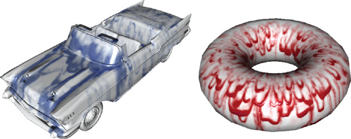
Figure 37-15 Liquid Flowing Along Mesh Surfaces
37.4 Conclusion
We have presented a complete GPU implementation of octree textures. These structures offer an efficient and convenient way of storing undistorted data along a mesh surface. This can be color data, as in the mesh-painting application, or data for dynamic texture simulation, as in the flowing liquid simulation. Rendering can be done efficiently on modern hardware, and we have provided solutions for filtering to avoid texture aliasing. Nevertheless, because 2D texture maps are preferable in some situations, we have shown how an octree texture can be dynamically converted into a 2D texture without artifacts.
Octrees are very generic data structures, widely used in computer science. They are a convenient way of storing information on unparameterized meshes, and more generally in space. Many other applications, such as volume rendering, can benefit from their hardware implementation.
We hope that you will discover many further uses for and improvements to the techniques presented in this chapter! Please see http://www.aracknea.net/octreetextures for updates of the source code and additional information.
37.5 References
Benson, D., and J. Davis. 2002. "Octree Textures." ACM Transactions on Graphics (Proceedings of SIGGRAPH 2002) 21(3), pp. 785–790.
Debry, D., J. Gibbs, D. Petty, and N. Robins. 2002. "Painting and Rendering Textures on Unparameterized Models." ACM Transactions on Graphics (Proceedings of SIGGRAPH 2002) 21(3), pp. 763–768.
Sander, P., J. Snyder, S. Gortler, and H. Hoppe. 2001. "Texture Mapping Progressive Meshes." In Proceedings of SIGGRAPH 2001, pp. 409–416.
Copyright
Many of the designations used by manufacturers and sellers to distinguish their products are claimed as trademarks. Where those designations appear in this book, and Addison-Wesley was aware of a trademark claim, the designations have been printed with initial capital letters or in all capitals.
The authors and publisher have taken care in the preparation of this book, but make no expressed or implied warranty of any kind and assume no responsibility for errors or omissions. No liability is assumed for incidental or consequential damages in connection with or arising out of the use of the information or programs contained herein.
NVIDIA makes no warranty or representation that the techniques described herein are free from any Intellectual Property claims. The reader assumes all risk of any such claims based on his or her use of these techniques.
The publisher offers excellent discounts on this book when ordered in quantity for bulk purchases or special sales, which may include electronic versions and/or custom covers and content particular to your business, training goals, marketing focus, and branding interests. For more information, please contact:
U.S. Corporate and Government Sales
(800) 382-3419
corpsales@pearsontechgroup.com
For sales outside of the U.S., please contact:
International Sales
international@pearsoned.com
Visit Addison-Wesley on the Web: www.awprofessional.com
Library of Congress Cataloging-in-Publication Data
GPU gems 2 : programming techniques for high-performance graphics and general-purpose
computation / edited by Matt Pharr ; Randima Fernando, series editor.
p. cm.
Includes bibliographical references and index.
ISBN 0-321-33559-7 (hardcover : alk. paper)
1. Computer graphics. 2. Real-time programming. I. Pharr, Matt. II. Fernando, Randima.
T385.G688 2005
006.66—dc22
2004030181
GeForce™ and NVIDIA Quadro® are trademarks or registered trademarks of NVIDIA Corporation.
Nalu, Timbury, and Clear Sailing images © 2004 NVIDIA Corporation.
mental images and mental ray are trademarks or registered trademarks of mental images, GmbH.
Copyright © 2005 by NVIDIA Corporation.
All rights reserved. No part of this publication may be reproduced, stored in a retrieval system, or transmitted, in any form, or by any means, electronic, mechanical, photocopying, recording, or otherwise, without the prior consent of the publisher. Printed in the United States of America. Published simultaneously in Canada.
For information on obtaining permission for use of material from this work, please submit a written request to:
Pearson Education, Inc.
Rights and Contracts Department
One Lake Street
Upper Saddle River, NJ 07458
Text printed in the United States on recycled paper at Quebecor World Taunton in Taunton, Massachusetts.
Second printing, April 2005
Dedication
To everyone striving to make today's best computer graphics look primitive tomorrow
- Copyright
- Inside Back Cover
- Inside Front Cover
- Part I: Geometric Complexity
-
- Chapter 1. Toward Photorealism in Virtual Botany
- Chapter 2. Terrain Rendering Using GPU-Based Geometry Clipmaps
- Chapter 3. Inside Geometry Instancing
- Chapter 4. Segment Buffering
- Chapter 5. Optimizing Resource Management with Multistreaming
- Chapter 6. Hardware Occlusion Queries Made Useful
- Chapter 7. Adaptive Tessellation of Subdivision Surfaces with Displacement Mapping
- Chapter 8. Per-Pixel Displacement Mapping with Distance Functions
- Part II: Shading, Lighting, and Shadows
-
- Chapter 9. Deferred Shading in S.T.A.L.K.E.R.
- Chapter 10. Real-Time Computation of Dynamic Irradiance Environment Maps
- Chapter 11. Approximate Bidirectional Texture Functions
- Chapter 12. Tile-Based Texture Mapping
- Chapter 13. Implementing the mental images Phenomena Renderer on the GPU
- Chapter 14. Dynamic Ambient Occlusion and Indirect Lighting
- Chapter 15. Blueprint Rendering and "Sketchy Drawings"
- Chapter 16. Accurate Atmospheric Scattering
- Chapter 17. Efficient Soft-Edged Shadows Using Pixel Shader Branching
- Chapter 18. Using Vertex Texture Displacement for Realistic Water Rendering
- Chapter 19. Generic Refraction Simulation
- Part III: High-Quality Rendering
-
- Chapter 20. Fast Third-Order Texture Filtering
- Chapter 21. High-Quality Antialiased Rasterization
- Chapter 22. Fast Prefiltered Lines
- Chapter 23. Hair Animation and Rendering in the Nalu Demo
- Chapter 24. Using Lookup Tables to Accelerate Color Transformations
- Chapter 25. GPU Image Processing in Apple's Motion
- Chapter 26. Implementing Improved Perlin Noise
- Chapter 27. Advanced High-Quality Filtering
- Chapter 28. Mipmap-Level Measurement
- Part IV: General-Purpose Computation on GPUS: A Primer
-
- Chapter 29. Streaming Architectures and Technology Trends
- Chapter 30. The GeForce 6 Series GPU Architecture
- Chapter 31. Mapping Computational Concepts to GPUs
- Chapter 32. Taking the Plunge into GPU Computing
- Chapter 33. Implementing Efficient Parallel Data Structures on GPUs
- Chapter 34. GPU Flow-Control Idioms
- Chapter 35. GPU Program Optimization
- Chapter 36. Stream Reduction Operations for GPGPU Applications
- Part V: Image-Oriented Computing
-
- Chapter 37. Octree Textures on the GPU
- Chapter 38. High-Quality Global Illumination Rendering Using Rasterization
- Chapter 39. Global Illumination Using Progressive Refinement Radiosity
- Chapter 40. Computer Vision on the GPU
- Chapter 41. Deferred Filtering: Rendering from Difficult Data Formats
- Chapter 42. Conservative Rasterization
- Part VI: Simulation and Numerical Algorithms
-
- Chapter 43. GPU Computing for Protein Structure Prediction
- Chapter 44. A GPU Framework for Solving Systems of Linear Equations
- Chapter 45. Options Pricing on the GPU
- Chapter 46. Improved GPU Sorting
- Chapter 47. Flow Simulation with Complex Boundaries
- Chapter 48. Medical Image Reconstruction with the FFT