
GPU Gems 2
GPU Gems 2 is now available, right here, online. You can purchase a beautifully printed version of this book, and others in the series, at a 30% discount courtesy of InformIT and Addison-Wesley.
The CD content, including demos and content, is available on the web and for download.
Chapter 36. Stream Reduction Operations for GPGPU Applications
Daniel Horn
Stanford University
Many GPGPU-based applications rely on the fragment processor, which operates across a large set of output memory locations, consuming a fixed number of input elements per location and operating a small program on those elements to produce a single output element in that location. Because the fragment program must write its results to a preordained memory location, it is not able to vary the amount of data that it outputs according to the input data it processes. (See Chapter 30 in this book, "The GeForce 6 Series GPU Architecture," for more details on the capabilities and limits of the fragment processor.)
Many algorithms are difficult to implement under these limitations—specifically, algorithms that reduce many data elements to few data elements. The reduction of data by a fixed factor has been carefully studied on GPUs (Buck et al. 2004); such operations require an amount of time linear in the size of the data to be reduced. However, nonuniform reductions—that is, reductions that filter out data based on its content on a per-element basis—have been less thoroughly studied, yet they are required for a number of interesting applications. We refer to such a technique of nonuniform reduction as a method of data filtering.
This chapter presents a data filtering algorithm that makes it possible to write GPU programs that efficiently generate varying amounts of output data.
36.1 Filtering Through Compaction
Assume we have a data set with arbitrary values and we wish to extract all positive values. On current GPUs, a fragment program that filters streams must produce null records for each output that should not be retained in the final output stream. Null records are represented with some value that the program will never generate when it does want to output a value. (In the examples that follow, we use floating-point infinity for this purpose. Floating-point infinity can be generated by computing 1.0/0.0, and it can be detected with the isinf() standard library function.) The following example uses the Brook programming language:
kernel void positive(float input<>, out float output<>, float inf<>)
{
  if (input > 0)
    output = input;
  else
    output = inf; // inf 1./0 must be passed in as a stream on ATI GPUs
}
The output must then be compacted, moving null records to the end. The most obvious method for compaction utilizes a stable sort to eliminate the null records; however, using bitonic sort to do this will result in a running time of O(n (log n)2) (Buck and Purcell 2004). Instead, we present a technique here that uses a scan (Hillis and Steele 1986) to obtain a running count of the number of null records, and then a search and gather to compact them, for a final running time of O(n log n).
36.1.1 Running Sum Scan
Given a list of data peppered with null records, to decide where a particular non-null record should redirect itself, it is sufficient to count the number of null records to the left of the non-null record, then move the record that many records to the left. On a parallel system, the cost of finding a running count of null records is actually O(n log n). The multipass technique to perform a running sum is called a scan. It starts by counting the number of nulls in the current record and the adjacent record exactly one index to the left, resulting in a number between 0 and 2 per record. This number is saved to a stream for further processing.
kernel void StartScan(float4 value[], out float count<>, iter float here<>,
                      iter float left_1<>)
{
  count = isinf(value[here].x) ? 1 : 0;
  if (here > = 1)
    count += isinf(value[left_1].x) ? 1 : 0;
}
Now each record in the stream holds the number of null records at its location and to the left of its location. This can be used to the algorithm's advantage in another pass, where the stream sums itself with records indexed two values to the left and saves the result to a new stream. Now each record in the new stream effectively has added the number of null records at zero, one, two, and three records to its left, because the record two items to the left in the previous stream already added the third item in the first pass. The subsequent steps add their values to values indexed at records of increasing powers of two to their left, until the power of two exceeds the length of the input array. This process is illustrated in Figure 36-1.
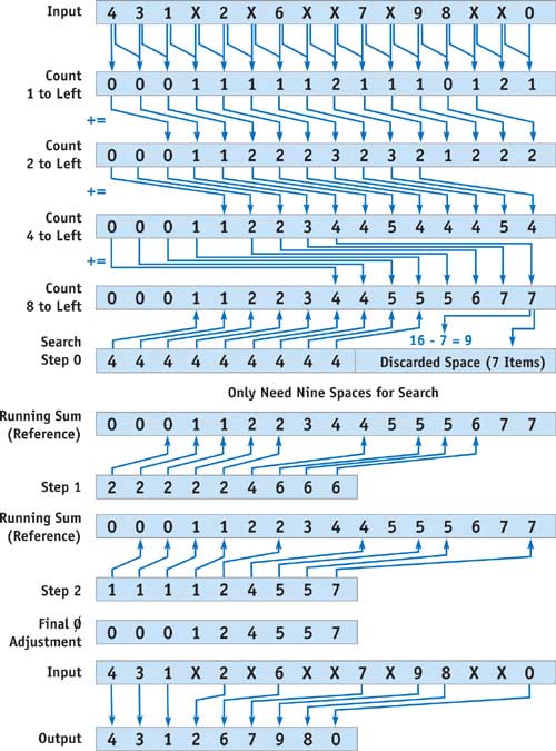
Figure 36-1 Iteratively Counting Null Records in a Stream
kernel void Scan(float input[], out float count<>, iter float here<>,
                 iter float left_2toi<>, float twotoi)
{
  count = input[here];
  if (here > twotoi)
    count += input[left_2toi];
}
After performing this multipass counting kernel log n times, each record knows how many nodes to the left to send its item. The value at the very right of the stream indicates how many null records there are in the entire stream, and hence the length of the compacted output, which is the total length minus the last value in the running sum stream. However, current fragment processors provide no way to send records, or scatter them, only to receive them with a texture fetch, or gather operation. Although vertex processors can scatter by rendering a stream of input points to various locations on the frame buffer, this does not make efficient use of the rasterizer.
36.1.2 Scatter Through Search/Gather
To overcome the lack of scatter on the fragment processor, we can use a parallel search algorithm to complete the filtering process. Luckily, a running sum is always monotonically increasing, so the result of the running sum scan step is a sorted, increasing set of numbers, which we can search to find the correct place from which to gather data.
Each record can do a parallel binary search, again in a total of O(log n) time to find the appropriate record from which to gather, using the running sum as a guide. This results in a total time of O(n log n) for n searches in parallel. If the running sum is equal to the distance from the current record to the record under consideration, then that record under consideration clearly wishes to displace its data to the current record; thus, the current record may just gather from it for the same effect. If the running sum is less, then the candidate record is too far to the right and must move left later in the algorithm. If the running sum is more than the distance, then the candidate must move to the right in the next iteration. Each iteration moves the candidate half as far away as the previous round until the current record narrows down the search to the actual answer. This search replaces the necessity of redirecting records (a scatter) and does not increase the asymptotic running time of O(n log n). See Listing 36-1.
Example 36-1. Search for Displaced Values Implemented in a Brook Kernel
kernel void GatherSearch(float scatterValues[], out float outGuess<>,
                         float4 value[], float twotoi, float lastguess<>,
                         iter float here<>)
{
  float guess = scatterValues[here + lastguess];
  float4 finalValue = value[here + lastguess];
  if (guess > lastguess)
    outGuess = lastguess + twotoi; // too low
  else if (guess == lastguess && !isinf(finalValue.x))
    outGuess = lastguess; // correct
  else
    outGuess = lastguess - twotoi; // too high
}
kernel void RelGather(out float4 outp<>, float gatherindex<>, float4 value[],
                      iter float here<>)
{
  outp = value[here + gatherindex];
}
The final result is obtained by gathering from the indices that the search located. Because the stream is already the correct size, the gathered values represent the filtered stream.
Optimization
On GPUs that support data-dependent looping or large numbers of instructions, there is an optimization that can make the parallel search cost negligible in comparison with the scan. The scan requires each subsequent pass to finish before using the results garnered from the pass; however, a search has no data dependency between passes and therefore may be completed in a single pass using dependent texture reads. See Listing 36-2.
Example 36-2. Using Looping to Search for Displaced Values
kernel void GatherSearch(float scatterValues[], out float4 output<>,
                         float4 value[],
                         float halfN, /* ceil(numNullElements/2+.5) */
                         float logN,
                         /* ceil(log(numNullElements)/log(2)) */
                         iter float here<>)
{
  float lastguess = halfN;
  float twotoi = halfN;
  float i;
  for (i = 0; i < logN; ++i)
  {
    float4 finalValue = value[here + lastguess];
    float guess = scatterValues[here + lastguess];
    twotoi /= 2;
    if (guess > lastguess)
      lastguess = lastguess + twotoi; // too low
    else if (guess == lastguess && !isinf(finalValue.x))
      lastguess = lastguess; // correct
    else
      lastguess = lastguess - twotoi; // too high
  }
  if (scatterValues[here] == 0)
    output = value[here];
  else
    output = value[here + lastguess];
}
On GPUs that do not support data-dependent loop limits, the kernel in Listing 36-2 may be compiled for each possible value of log2 n for the given application.
36.1.3 Filtering Performance
To measure whether the scan/search algorithm is faster than the bitonic sort, we implemented both algorithms in Brook using 1D-to-2D address translation and the same programming style. Scan is almost exactly 0.5 x log2 n times faster than a bitonic sort, because bitonic sort requires a factor of 0.5 x (log2 n - 1) extra passes and has a similar number of instructions and pattern of memory access. In Table 36-1, we see how many microseconds it takes to filter each element on various hardware.
Table 36-1. Timing of Compaction Methods on Modern Hardware
|
In s per record (lower is better). |
||||||||
|
Number of Records |
||||||||
|
64k |
128k |
256k |
512k |
1024k |
2048k |
4096k |
||
|
6800 Ultra |
Scan/Search |
0.138 |
0.131 |
0.158 |
0.151 |
0.143 |
0.167 |
0.161 |
|
6800 Ultra |
Bitonic Sort |
1.029 |
0.991 |
1.219 |
1.190 |
1.455 |
1.593 |
1.740 |
|
X800 |
Scan/Search |
0.428 |
0.267 |
0.288 |
0.355 |
0.182 |
0.169 |
0.168 |
|
X800 |
Bitonic Sort |
0.762 |
0.912 |
0.968 |
1.051 |
1.175 |
1.269 |
1.383 |
Clearly the scan/search filtering method illustrated here is more efficient than sorting. Although the cost per element is not constant in data size, as is the same operation on the CPU, the cost does not increase much as the data size increases exponentially. Note that the looping construct is used to perform the parallel search on the NVIDIA GeForce 6800 Ultra, which gives it an added advantage over the bitonic sort on that hardware.
36.2 Motivation: Collision Detection
To see the utility of this filtering idiom, consider search algorithms based on tree traversal, for example, the University of North Carolina's RAPID hierarchical bounding volume collision-detection scheme (Gottschalk et al. 1996). The basic idea is that two trees of bounding volumes for two models may be traversed in unison to find overlapping volumes and eventually overlapping leaf nodes, which contain potentially touching triangles. Fast collision detection among rigid meshes is important for many graphics applications. For instance, haptic rendering, path planning, and scene interaction all require this form of collision detection.
We begin by porting an algorithm to perform collision detection to the streaming language Brook (Buck et al. 2004). The inputs to the collision-detection scheme are two triangulated 3D models, and a rigid transformation between the two; the output is a list of pairs of triangles that overlap. An offline computation creates a tree of bounding boxes for each 3D model, starting from a top-level bounding box containing that whole model. The tree is created such that each bounding box node either has two smaller bounding boxes within it, or else is a leaf node containing a pointer to a single triangle from the input model. This tree may be downloaded to the GPU for online collision-detection processing. Each bounding box contains a rigid transformation, a size, and a pointer to its children. In Brook, for each model, we may make two streams of structures that contain this static information: one for the list of triangles and the other for the hierarchy of bounding boxes that encloses them. See Listing 36-3.
Example 36-3. Data Structures for Collision Detection
typedef struct Tri_t
{
  float3 A, B, C;
} Tri;
typedef struct bbox_t
{
  float4 Rotationx; // The x axis of the bounding box coordinate system
  // Rotationx.w -1 for left-handed coordinate system
  float3 Rotationy; // The y axis of the bounding box coordinate system
  // float3 Rotationz; // since Rotationx and Rotationy are orthogonal
  // use cross(Rotationx,Rotationy)*Rotationx.w;
  float3 Translation;
  // the bottom corner of the bounding box
  float4 Radius; // The dimensions of the bounding box
  // Radius.w holds bool whether this node is a leaf
  float2 Children;
  // if leaf, Children.xy is an index to the Triangle in the model
  // if node, Children.xy is an index to left child,
  //
  Children.xy + float2(1, 0) is right child
} BBox;
To determine which triangles overlap in the two models, we process the trees of bounding boxes breadth-first. A stream of candidate pairs is processed, and pairs that can be trivially rejected because their bounding boxes do not intersect are dropped from the stream. Pairs that cannot be rejected are divided into a set of pairs of child nodes. The process is repeated until only leaf nodes remain. This process requires removing some pairs from the stream and inserting others. It would be impractical to start with a stream of maximum necessary length and ignore elements that do not collide, because doing so loses the advantages of the tree traversal and pruning process.
For example, to determine which triangles overlap in the two models A and B, we begin with the largest bounding boxes that form the root of each of the two trees in the input models. Suppose model A is a small model that has bounding box root Ra and model B is a larger model with bounding box root Rb . We will first check if Ra overlaps with Rb , and if not, then there must be no collision, because the entire models are contained in Ra and Rb , respectively. Assuming that Ra and Rb overlap, we take the two children of the larger bounding box Cb and Db and compare each in turn with Ra to check for overlap. We can repeat this procedure, checking Ra 's children Ca and Da with the potential colliders from Cb and Db , splitting each bounding box into its two components at each phase until we reach leaf nodes that point to actual triangles. Finally, we compare the pairs of triangles contained in each overlapping leaf node with each other, checking for collisions. See Figure 36-2. On average, far fewer leaf nodes are processed with this approach than there are pairs of triangles, but it is easily conceivable that a pair of degenerate models could be designed such that each triangle must be checked with each other triangle in the two models.
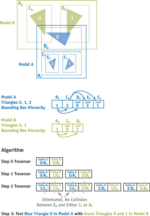
Figure 36-2 Collision Detection with Two Bounding Box Trees
A data structure to contain the dynamic state needed for the traversal of the node hierarchies could thus be contained in the following:
typedef struct traverser_t
{
  float4 index; // index.xy is index into the first model
  // index.zw is index into the second model
  float3 Translation;
  float3 Rotationx;
  float3 Rotationy;
  float3 Rotationz;
} Traverser;
In Listing 36-4, we examine some CPU pseudocode to check collisions on two given models, with the preceding data structures.
Porting Collision Detection to the GPU
Now that we have established a systematic method for searching the pair of trees for triangle intersections, the question remains how to best implement this algorithm as a fragment program on the graphics hardware. To do so, a breadth-first search on a tree may be represented as follows: At any given stage of the algorithm, a stream of candidate pairs of bounding box nodes for a collision may be checked in parallel. Pairs of candidates that clearly do not collide must be filtered, and overlapping pairs of bounding boxes must be split, one for each child node of the larger bounding box. Another pass may be made on the filtered and split candidate pairs until only leaf nodes remain. Those leaf nodes may be checked for actual geometry collisions.
Example 36-4. Collision Pseudocode
bool collide(BBox mA[], BBox mB[], Triangle tri[], Traverser state)
{
  BBox A = mA[state.index.xy] BBox B =
      mB[state.index.zw] if (bb_overlap(state, A.Radius, B.Radius))
  {
    if (isLeaf(A) && isLeaf(B))
    {
      return tri_overlap(tri[A.Children], tri[B.Children])
    }
    else
    {
      if (AisBigger(A, B))
      { // bigger or nonleaf
        state = Compose(state, A.Translation, A.Rotationx, A.Rotationy);
        state.index.xy = LeftChild(A);
        bool ret = collide(mA, mB, tri, state);
        state.index.xy = RightChild(A);
        return ret || collide(mA, mB, tri, state);
      }
      else
      { // B is bigger than A or A is a leaf node
        state = invCompose(state, B.Translation, B.Rotationx, B.Rotationy);
        state.index.zw = LeftChild(B);
        bool ret = collide(mA, mB, tri, state);
        state.index.zw = RightChild(B);
        return ret || collide(mA, mB, tri, state);
      }
    }
  }
  return false;
}
Thus, given a filtering operator primitive, the overall collision-detection algorithm itself runs as follows, depicted in Figure 36-2. Starting from a single pair of top-level bounding boxes for the models in question, each active bounding box pair is checked for collision. Next, bounding box pairs that do not collide are filtered out using the filtering primitive described in Section 36.1. The short list of remaining pairs of leaf bounding boxes that point to triangles in the respective models are checked for physical collision. The remaining list of nonleaf pairs is doubled in length, one for each child of the larger of the two bounding boxes. The algorithm is then repeated for this doubled list, until it has been filtered to length zero.
36.3 Filtering for Subdivision Surfaces
The filtering idiom we presented is useful not only in tree searches such as collision detection, but also in conjunction with imbalanced trees, graphs, and other sparse data sets such as meshes. A hardware-accelerated adaptive subdivision surface tessellation algorithm offers an interesting possibility as the computational capabilities of fragment programs continue to improve. Subdivision surfaces operate as follows: Given an input mesh with connectivity information, an output mesh of four times the number of triangles is produced. Each triangle is then split into four smaller triangles, and those triangles' vertex positions are updated based on neighboring vertex positions. The result is a smoother mesh. Repetition of this algorithm causes the mesh to converge to a smooth limit surface.
Adaptive subdivision surfaces operate similarly, but with the caveat that some triangles may be frozen based on image-space size, curvature, or any per-edge constraint, and hence not divided. In this case, we examine Loop's subdivision scheme (Loop 1987), which uses neighbor information from the adjacent polygons to compute a smoothed vertex position. This process may be repeated until the desired polygon count is reached. In the limiting case, Loop subdivision guarantees C2 continuity at vertices that have six neighbors and hence a valence of six; it guarantees C1 continuity at the vertices that have a valence other than six. A surface with C1 continuity has no sharp corners, and a surface with C2 continuity has no drastic changes in curvature along that surface. Loop subdivision never creates new vertices with higher valence than the original model, so the original model dictates the highest possible valence.
36.3.1 Subdivision on Streaming Architectures
We implement adaptive subdivision surfaces in Brook using the filtering process presented in Section 36.1. An adaptive subdivision scheme requires filtering completed triangles at each stage of the algorithm, and it requires communication to determine which neighbors are filtered.
In a streaming application that operates on a stream of triangles of increasing sparseness, it is prudent to have each triangle be self-contained, tracking the coordinates of its neighboring vertices, instead of saving and updating indices to neighbors. The texture indirection from its neighbor list, and the as-yet-unsolved problem of tracking updates to the neighbor list as subdivision continues, make tracking pointers to neighbors a difficult proposition. However, tracking the coordinates of neighbors directly uses only a quarter more storage and results in far fewer dependent texture lookups and thus faster performance.
The algorithm operates on a stream of triangles, consisting of three coordinates per vertex, and a Boolean value indicating if any edge that the vertex touches has completed its subdivision. Alongside this stream of triangles is a stream of neighboring vertices, consisting of nine vertices arranged in a clockwise ordering, as illustrated in Figure 36-3. Thus, we assert a maximum valence of six for code brevity, though no such limit is imposed by the algorithm in general. After a triangle is split, the floats in the neighbor list refer to differing items based on the extra three neighboring vertices that are created during the split. A separate split-triangle structure is used to contain the six split and perturbed vertices within the original triangle. See Listing 36-5.
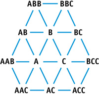
Figure 36-3 Triangle ABC and Its Neighbors
Example 36-5. Data Structures for Subdivision
typedef struct STri_t
{
  float4 A; // A.w indicates whether edge AB may stop subdivision
  float4 B; // B.w also indicates if BC may stop subdivision
  float4 C; // C.w tells if AC is small enough to stop subdividing
} STri;
// Stores the neighbors of a given triangle.
// The extra w component holds:
// a) whether respective edge may stop subdividing of triangle.
//
This could be altered to any per -
    edge qualifier.
    // b) or for the intermediate triangle split, the recomputed
    //
    averaged neighbor list when a triangle is split typedef struct Neighbor_t
{
  float4 AB;
  // AB.w = avg(AB,B).x
  float4 BBC; // BBC.w = avg(AB,B).y
  float4 ABB; // ABB.w = avg(AB,B).z
  float4 BC;
  // BC.w = avg(BC,C).x
  float4 ACC; // ACC.w = avg(BC,C).y
  float4 BCC; // BCC.w = avg(BC,C).z
  float4 AC;
  // AC.w = avg(AC,A).x
  float4 AAB; // AAB.w = avg(AC,A).y
  float4 AAC; // AAC.w = avg(AC,A).z
} Neighbor;
The initial data is given as two streams: a stream of triangles forming a closed mesh and a stream of neighbors to the triangles that make up the first stream. Triangle edges are each checked in turn for completion, and the stream is filtered for completed triangles. These triangles are saved for rendering, and the inverse filter is applied to the list to determine which triangles are in need of further subdivision. For nonadaptive subdivision, the filter stage can be replaced with a polygon count check to terminate subdivision altogether.
When a triangle is completed but its neighbors are not, a T-junction can appear where the edge of one triangle abuts a vertex of another. These need to be patched so as to preserve the mesh's state of being closed. At each stage, T-junctions can be detected by measuring whether two edges of a vertex have reached the exit condition, even if the triangle in question is still subdividing. When a T-junction is detected, our implementation has opted to place a sliver triangle there, filling in the potential rasterization gap between the polygons that have a T-junction. Other techniques, such as Red-Green triangulation (Seeger et al. 2001), may make more pleasing transitions, but this choice was made for its simplicity.
Finally, the subdivision calculation stage occurs. Each vertex in the triangle stream is weighted by its neighbors and split according to Loop's subdivision rule, resulting in six vertices per triangle: three near the original triangle corners and three new ones near the midpoints of the original triangle edges. The neighbors are likewise split, and the resulting 12 vertices are spread over the nine float4 values. To recurse on this data, new streams are made that are four times as long as the split triangle and split neighbor streams. The new values are ordered into the appropriate original Neighbor and Triangle structures, depending on the arithmetic remainder of the output index divided by four. At this point, Boolean values declaring whether the edges of the triangle in question meet the per-edge constraint are computed, giving a hint to the filtering stage in the next round. The algorithm is repeated until a maximum depth is reached, or until all triangles have been filtered out as complete.
Details Specific to Streaming on the GPU
There are a few caveats that should be noted: Each of the triangles surrounding a given vertex must make the same decision about where the vertex ends up. This requires a few cautionary practices. First, vertices that are currently in the mesh must be weighted independently by all neighbors. Because floating-point addition is not associative, the surrounding values must be sorted from smallest to largest before being added together. This results in each of the triangles containing a vertex making the same decision about the final location of that vertex. Second, some optimizing compilers do not always respect IEEE floating-point standards in their optimizations and may reorder floating-point operations in ways that break the commutativity of floating-point addition. Others, like the Cg compiler, provide a command-line switch to control this behavior.
36.4 Conclusion
In this chapter we have demonstrated the utility of a filtering idiom for graphics hardware. The filtering paradigm enables a number of new applications that operate by filtering a data set at the price of a scan and search. Searching is becoming faster due to the recent addition of branching and looping to vertex programs, yet improvement of the scanning phase of the algorithm is largely predicated on having new hardware. Specifically, a central running sum register that can quickly produce unique, increasing values for fragments to use, and the ability to send fragments to other locations in the frame buffer would allow for a linear-time scan phase, and then would result in a direct output of the appropriate values. However, using a running sum register would destroy any order of the filtered fragments. The order has, however, been largely unnecessary in the algorithms presented here.
Future hardware has the distinct possibility of supporting order-preserving filtering natively and offers an exciting possibility for improving performance of general-purpose programmability.
There are plenty of other applications that can benefit from this idiom. For example, Monte Carlo ray tracing produces zero, one, or more rays per intersection with a surface. The scene may be traversed using the filtering idiom described in this chapter to propagate rays, terminating them when necessary, and producing more after an intersection. Marching Cubes takes a large 3D data set and culls it down into a 2D surface of interest, weighting the triangle vertices by the measured density values. An example of the Marching Cubes algorithm utilizing filtering is included with the Brook implementation available online at the Brook Web site (Buck et al. 2004). Furthermore, as shown by our collision-detection application, filtering permits GPUs to traverse tree data structures. This same approach could be used with other applications that operate on trees.
36.5 References
To learn more about collisions on the GPU, see the published papers on how to do collision detection on GPUs. A majority of the algorithms operate in image space, selecting views from which to render two objects such that colliding objects overlap. These algorithms, although fast in practice, often rely heavily on fine sampling to cull enough work away initially. They require O(n) time, where n is the sum total of polygons in their objects (Govindaraju et al. 2003).
Hierarchical schemes are on average asymptotically faster. Gress and Zachmann (2003) also devised an object-space scheme for hierarchical collision detection, instead of a balanced tree of axis-aligned bounding boxes. They perform a breadth-first search into the respective collision trees, but at each level they use occlusion query to count the number of overlapping bounding boxes at that level. They allocate a texture of the appropriate size and search for the sequential filtered list of bounding boxes using a progressively built balanced tree structure. This technique, requiring O(log n) extra passes over the data to perform filtering effectively, emulates the technique presented in this chapter, but it is limited in scope to collision detection on balanced trees, instead of a more generic filtering technique.
Likewise, for more information on tessellation of subdivision surfaces, Owens et al. (2002) presented adaptive Catmull-Clark quadrilateral subdivision on the Imagine processor using a technique similar to the one presented in this chapter, but that algorithm utilized the conditional move operation present in the Imagine processor architecture (Khailany et al. 2001), which provides data filtering in hardware.
Buck, I., T. Foley, D. Horn, J. Sugarman, and P. Hanrahan. 2004. "Brook for GPUs: Stream Computing on Graphics Hardware." ACM Transactions on Graphics (Proceedings of SIGGRAPH 2004) 23(3). Available online at http://graphics.stanford.edu/projects/brookgpu/
Buck, I., and T. Purcell. 2004. "A Toolkit for Computation on GPUs." In GPU Gems, edited by Randima Fernando, pp. 621–636.
Gottschalk, S., M. C. Lin, and D. Manocha. 1996. "OBB-Tree: A Hierarchical Structure for Rapid Interference Detection." In Proceedings of SIGGRAPH 96, pp. 171–180.
Govindaraju, N. K., S. Redon, M. C. Lin, and D. Manocha. 2003. "CULLIDE: Interactive Collision Detection Between Complex Models in Large Environments Using Graphics Hardware." In Proceedings of the SIGGRAPH/Eurographics Workshop on Graphics Hardware 2003, pp. 25–32.
Gress, A., and G. Zachmann. 2003. "Object-Space Interference Detection on Programmable Graphics Hardware." In Proceedings of the SIAM Conference on Geometric Design and Computing, pp. 13–17.
Hillis, W. D., and G. L. Steele, Jr. 1986. "Data Parallel Algorithms." Communications of the ACM 29(12), p. 139.
Khailany, B., W. J. Dally, et al. 2001. "Imagine: Media Processing with Streams." IEEE Micro, March/April 2001.
Loop, C. 1987. "Smooth Subdivision Surfaces Based on Triangles." Master's thesis, Department of Mathematics, University of Utah.
Owens, J. D., B. Khailany, B. Towles, and W. J. Dally. 2002. "Comparing Reyes and OpenGL on a Stream Architecture." In Proceedings of the SIGGRAPH/Eurographics Workshop on Graphics Hardware, pp. 47–56.
Seeger, S., K. Hormann, G. Hausler, and G. Greiner. 2001. "A Sub-Atomic Subdivision Approach." In Proceedings of the Vision, Modeling, and Visualization Conference.
Copyright
Many of the designations used by manufacturers and sellers to distinguish their products are claimed as trademarks. Where those designations appear in this book, and Addison-Wesley was aware of a trademark claim, the designations have been printed with initial capital letters or in all capitals.
The authors and publisher have taken care in the preparation of this book, but make no expressed or implied warranty of any kind and assume no responsibility for errors or omissions. No liability is assumed for incidental or consequential damages in connection with or arising out of the use of the information or programs contained herein.
NVIDIA makes no warranty or representation that the techniques described herein are free from any Intellectual Property claims. The reader assumes all risk of any such claims based on his or her use of these techniques.
The publisher offers excellent discounts on this book when ordered in quantity for bulk purchases or special sales, which may include electronic versions and/or custom covers and content particular to your business, training goals, marketing focus, and branding interests. For more information, please contact:
U.S. Corporate and Government Sales
(800) 382-3419
corpsales@pearsontechgroup.com
For sales outside of the U.S., please contact:
International Sales
international@pearsoned.com
Visit Addison-Wesley on the Web: www.awprofessional.com
Library of Congress Cataloging-in-Publication Data
GPU gems 2 : programming techniques for high-performance graphics and general-purpose
computation / edited by Matt Pharr ; Randima Fernando, series editor.
p. cm.
Includes bibliographical references and index.
ISBN 0-321-33559-7 (hardcover : alk. paper)
1. Computer graphics. 2. Real-time programming. I. Pharr, Matt. II. Fernando, Randima.
T385.G688 2005
006.66—dc22
2004030181
GeForce™ and NVIDIA Quadro® are trademarks or registered trademarks of NVIDIA Corporation.
Nalu, Timbury, and Clear Sailing images © 2004 NVIDIA Corporation.
mental images and mental ray are trademarks or registered trademarks of mental images, GmbH.
Copyright © 2005 by NVIDIA Corporation.
All rights reserved. No part of this publication may be reproduced, stored in a retrieval system, or transmitted, in any form, or by any means, electronic, mechanical, photocopying, recording, or otherwise, without the prior consent of the publisher. Printed in the United States of America. Published simultaneously in Canada.
For information on obtaining permission for use of material from this work, please submit a written request to:
Pearson Education, Inc.
Rights and Contracts Department
One Lake Street
Upper Saddle River, NJ 07458
Text printed in the United States on recycled paper at Quebecor World Taunton in Taunton, Massachusetts.
Second printing, April 2005
Dedication
To everyone striving to make today's best computer graphics look primitive tomorrow
- Copyright
- Inside Back Cover
- Inside Front Cover
- Part I: Geometric Complexity
-
- Chapter 1. Toward Photorealism in Virtual Botany
- Chapter 2. Terrain Rendering Using GPU-Based Geometry Clipmaps
- Chapter 3. Inside Geometry Instancing
- Chapter 4. Segment Buffering
- Chapter 5. Optimizing Resource Management with Multistreaming
- Chapter 6. Hardware Occlusion Queries Made Useful
- Chapter 7. Adaptive Tessellation of Subdivision Surfaces with Displacement Mapping
- Chapter 8. Per-Pixel Displacement Mapping with Distance Functions
- Part II: Shading, Lighting, and Shadows
-
- Chapter 9. Deferred Shading in S.T.A.L.K.E.R.
- Chapter 10. Real-Time Computation of Dynamic Irradiance Environment Maps
- Chapter 11. Approximate Bidirectional Texture Functions
- Chapter 12. Tile-Based Texture Mapping
- Chapter 13. Implementing the mental images Phenomena Renderer on the GPU
- Chapter 14. Dynamic Ambient Occlusion and Indirect Lighting
- Chapter 15. Blueprint Rendering and "Sketchy Drawings"
- Chapter 16. Accurate Atmospheric Scattering
- Chapter 17. Efficient Soft-Edged Shadows Using Pixel Shader Branching
- Chapter 18. Using Vertex Texture Displacement for Realistic Water Rendering
- Chapter 19. Generic Refraction Simulation
- Part III: High-Quality Rendering
-
- Chapter 20. Fast Third-Order Texture Filtering
- Chapter 21. High-Quality Antialiased Rasterization
- Chapter 22. Fast Prefiltered Lines
- Chapter 23. Hair Animation and Rendering in the Nalu Demo
- Chapter 24. Using Lookup Tables to Accelerate Color Transformations
- Chapter 25. GPU Image Processing in Apple's Motion
- Chapter 26. Implementing Improved Perlin Noise
- Chapter 27. Advanced High-Quality Filtering
- Chapter 28. Mipmap-Level Measurement
- Part IV: General-Purpose Computation on GPUS: A Primer
-
- Chapter 29. Streaming Architectures and Technology Trends
- Chapter 30. The GeForce 6 Series GPU Architecture
- Chapter 31. Mapping Computational Concepts to GPUs
- Chapter 32. Taking the Plunge into GPU Computing
- Chapter 33. Implementing Efficient Parallel Data Structures on GPUs
- Chapter 34. GPU Flow-Control Idioms
- Chapter 35. GPU Program Optimization
- Chapter 36. Stream Reduction Operations for GPGPU Applications
- Part V: Image-Oriented Computing
-
- Chapter 37. Octree Textures on the GPU
- Chapter 38. High-Quality Global Illumination Rendering Using Rasterization
- Chapter 39. Global Illumination Using Progressive Refinement Radiosity
- Chapter 40. Computer Vision on the GPU
- Chapter 41. Deferred Filtering: Rendering from Difficult Data Formats
- Chapter 42. Conservative Rasterization
- Part VI: Simulation and Numerical Algorithms
-
- Chapter 43. GPU Computing for Protein Structure Prediction
- Chapter 44. A GPU Framework for Solving Systems of Linear Equations
- Chapter 45. Options Pricing on the GPU
- Chapter 46. Improved GPU Sorting
- Chapter 47. Flow Simulation with Complex Boundaries
- Chapter 48. Medical Image Reconstruction with the FFT