
GPU Gems 2
GPU Gems 2 is now available, right here, online. You can purchase a beautifully printed version of this book, and others in the series, at a 30% discount courtesy of InformIT and Addison-Wesley.
The CD content, including demos and content, is available on the web and for download.
Chapter 24. Using Lookup Tables to Accelerate Color Transformations
Jeremy Selan
Sony Pictures Imageworks
In feature-film visual-effects production, maintaining interactive feedback of high-quality color operations is extraordinarily beneficial to an artist. On the consumer side, enabling the real-time color correction of video and rendered image streams is becoming an increasingly useful tool to shape media's thematic "look." However, directly applying multiple sophisticated color transforms to high-resolution imagery is beyond the real-time capability of modern graphics hardware.
In this chapter, we present an algorithm that leverages three-dimensional lookup tables to enable the real-time color processing of high-resolution imagery. Our approach offers excellent performance characteristics, being independent of both the number of color operators applied as well as the underlying color transform complexity. The techniques presented in this chapter, and variations thereof, have been successfully utilized in the production of numerous motion pictures and should be regarded as "production ready."
24.1 Lookup Table Basics
Lookup tables (LUTs) are an excellent technique for optimizing the evaluation of functions that are expensive to compute and inexpensive to cache. By precomputing the evaluation of a function over a domain of common inputs, expensive runtime operations can be replaced with inexpensive table lookups. If the table lookups can be performed faster than computing the results from scratch (or if the function is repeatedly queried at the same input), then the use of a lookup table will yield significant performance gains. [1] For data requests that fall between the table's samples, an interpolation algorithm can generate reasonable approximations by averaging nearby samples.
24.1.1 One-Dimensional LUTs
A lookup table is characterized by its dimensionality, that is, the number of indices necessary to index an output value. The simplest LUTs are indexed by a single variable and thus referred to as one-dimensional (or 1D) LUTs.
The identity lookup table is defined as the transform that maps the input index back to itself over a given domain, as shown in Figure 24-1.
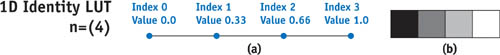
Figure 24-1 How One-Dimensional Lookup Tables Work
One-dimensional LUTs have long been utilized in image processing, most commonly in the form of the monitor gamma table. Typically leveraging three LUTs—one for each color channel—these tables enable the computationally efficient modification of pixel intensity just before an image reaches the monitor.
Consider an analytical color operator, f(x), applied to an 8-bit grayscale image. The naive implementation would be to step through the image and for each pixel to evaluate the function. However, one may observe that no matter how complex the function, it can evaluate to only one of 255 output values (corresponding to each unique input). Thus, an alternate implementation would be to tabulate the function's result for each possible input value, then to transform each pixel at runtime by looking up the stored solution. Assuming that integer table lookups are efficient (they are), and that the rasterized image has more than 255 total pixels (it likely does), using a LUT will lead to a significant speedup.
All color operators that can be parameterized on a single input variable can be accelerated using 1D LUTs, including the brightness, gamma, and contrast operators. See Figure 24-2. By assigning a 1D LUT to each color channel individually, we can implement more sophisticated operations, such as color balancing. For those familiar with the Photoshop image-processing software, all "Curves" and "Levels" operations can be accelerated with 1D LUTs.
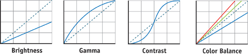
Figure 24-2 A Variety of Simple Color Operators
Limitations of 1D LUTs
Unfortunately, many useful color operators cannot be parameterized on a single variable, and are thus impossible to implement using a single-dimensional LUT. For example, consider the "luminance operator" that converts colored pixels into their grayscale equivalent. Because each output value is derived as a weighted average of three input channels, one would be hard-pressed to express such an operator using a 1D LUT. All other operators that rely on such channel "cross talk" are equally inexpressible.
24.1.2 Three-Dimensional LUTs
Three-dimensional lookup tables offer the obvious solution to the inherent limitation of single-dimensional LUTs, allowing tabular data indexed on three independent parameters, as shown in Figure 24-3.
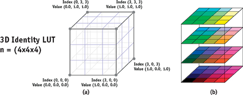
Figure 24-3 A Three-Dimensional Lookup Table
Whereas a 1D LUT requires only 4 elements to sample 4 locations per axis, the corresponding 3D LUT requires 43 = 64 elements. Beware of this added dimensionality; 3D LUTs grow very quickly as a function of their linear sampling rate. [2] As a direct implication of smaller LUT sizes, high-quality interpolation takes on a greater significance for 3D LUTs, as opposed to the 1D realm, where simple interpolators are often practical.
Complex color operators can be expressed using 3D LUTs, as completely arbitrary input-output mappings are allowed. For this reason, 3D LUTs have long been embraced by the colorimetry community and are one of the preferred tools in gamut mapping (Kang 1997). In fact, 3D LUTs are used within ICC profiles to model the complex device behaviors necessary for accurate color image reproduction (ICC 2004).
The majority of color operators are expressible using 3D LUTs. Simple operators (such as gamma, brightness, and contrast) are trivial to encode. More complex transforms, such as hue and saturation modifications, are also possible. Most important, the color operations typical of professional color-grading systems are expressible (such as the independent warping of user-specified sections of the color gamut). See Figure 24-4.
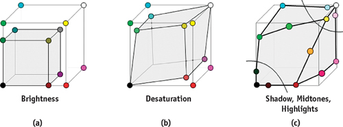
Figure 24-4 Simulating Color Transforms with Three-Dimensional Lookup Tables
Limitations of 3D LUTs
Unfortunately, in real-world scenarios, not all color transforms are definable as direct input-output mappings. In the general case, 3D LUTs can express only those transforms that obey the following characteristics:
- A pixel's computation must be independent of the spatial image position. Color operators that are influenced by neighboring values, such as Bayesian-matting (Chuang et al. 2001) or garbage masks (Brinkman 1999), are not expressible in lookup-table form.
- The color transform must be reasonably continuous, as sparsely sampled data sets are ill suited to represent discontinuous transformations. If smoothly interpolating over the sampled transform grid yields unacceptable results, lookup tables are not the appropriate acceleration technique.
- The input color space must lie within a well-defined domain. An "analytically" defined brightness operator can generate valid results over the entire domain of real numbers. However, that same operator baked into a lookup table will be valid over only a limited domain (for example, perhaps only in the range [0,1]). Section 24.2.4 addresses ways to mitigate this issue.
24.1.3 Interpolation
Interpolation algorithms allow lookup tables to generate results when queried for values between sample points. The simplest method, nearest-neighbor interpolation, is to find and return the nearest table entry. Although this method is fast (requiring only a single lookup), it typically yields discontinuous results and is thus rarely utilized in image processing.
A more advanced interpolation algorithm is to compute the weighted average between the two bounding samples (in the case of 1D LUTs), based on the relative distance of the sample to its neighbors. Known as linear interpolation, this approach provides significantly smoother results than the nearest-neighbor scheme.
Linear interpolation is adapted to 3D data sets by successively applying 1D linear interpolation along each of the three axes (hence the designation trilinear interpolation). By generating intermediate results based on a weighted average of the eight corners of the bounding cube, this algorithm is typically sufficient for color processing, and it is commonly implemented in graphics hardware. Higher-order interpolation functions use progressively more samples in the reconstruction function, though at significantly higher computation costs. (Straightforward cubic interpolation requires 33 = 27 texture lookups, but see Chapter 20 of this book, "Fast Third-Order Texture Filtering," for a technique that reduces this to 8 lookups.)
24.2 Implementation
Our approach is based on the assumption that it is cheap to trilinearly interpolate 3D textures. Whereas this is decidedly not true for software implementations, we can leverage the 3D texturing capabilities of modern GPUs to function as our color-correction engine.
24.2.1 Strategy for Mapping LUTs to the GPU
Most modern GPUs offer hardware-accelerated trilinear, 3D texture lookups (the interpolation unit was originally necessary for mipmapped, 2D texture lookups); thus, our algorithm becomes fairly trivial to implement.
First, we load our high-resolution image into a standard 2D texture. Next, we load our 3D color correction mapping as a 3D texture, being careful to enable trilinear filtering (in OpenGL this requires the texture magnification filter set to GL_LINEAR).
At runtime, we transform our input image by sampling the color in the normal fashion and then by performing a dependent texture lookup into the 3D texture (using the result of the 2D texture lookup as the 3D texture's input indices). The output of the 3D texture is our final, color-transformed result.
24.2.2 Cg Shader
The fragment shader code, shown in Listing 24-1, is almost as simple as you would expect. The efficiency of this approach is readily apparent, as the entire color-correction process is reduced to a single (3D) texture lookup.
Example 24-1. Fragment Shader to Perform the 3D Texture Lookup
void main(in float2 sUV
          : TEXCOORD0, out half4 cOut
          : COLOR0, const uniform samplerRECT imagePlane,
            const uniform sampler3D lut, const uniform float3 lutSize)
{
  // Get the image color
  half3 rawColor = texRECT(imagePlane, sUV).rgb;
  // Compute the 3D LUT lookup scale/offset factor
  half3 scale = (lutSize - 1.0) / lutSize;
  half3 offset = 1.0 / (2.0 * lutSize);
  // ****** Apply 3D LUT color transform! **************
  // This is our dependent texture read; The 3D texture's
  // lookup coordinates are dependent on the
  // previous texture read's result
  cOut.rgb = tex3D(lut, scale * rawColor + offset);
}
Shader Analysis
The most common question is probably "Why are the scale and offset factors necessary?" The answer relates to the coordinate system that the texture-mapping hardware uses to sample from our LUT. Specifically, the hardware texture-sampling algorithms sample (by default) from one extreme of the data set to the other. Though this is entirely reasonable when texturing image data, it is not appropriate for sampling numerical data sets, because it introduces nonlinearities near the texture's edges, as shown in Figure 24-5. Thus, to properly interpolate our "data" image, we must query only the region between the outer sample's centers, according to the following equation:
|
Adjusted sample coordinate = (lutSize - 1.0)/lutSize x oldCoord + 1.0/(2.0 x lutSize) |
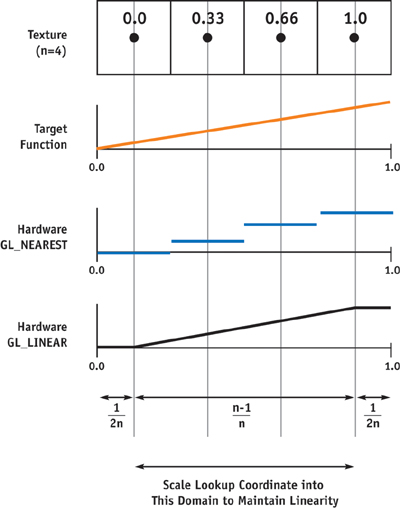
Figure 24-5 Problems Caused by Uncorrected Linear Interpolation
Observe that as the size of the LUT grows large, the correction factor becomes negligible. For example, with a 4,096-entry lookup table (a common 1D LUT size), the scaling factor can be safely ignored, as the error is smaller than the precision of the half pixel format. However, for the small lattice sizes common to 3D LUTs, the effect is visually significant and cannot be ignored; uncorrected 8-bit scaling errors on a 32x32x32 LUT are equivalent to clamping all data outside of [4..251]!
Shader Optimization
This code has obvious acceleration opportunities. First, as the scale and offset factors are constant across the image, they can be computed once and passed in as constants. (Or even better, they can be directly compiled into the fragment shader.) Second, it is good practice to use the smallest LUT that meets your needs (but no smaller). For "primary grading" color corrections, where one only modifies the color of the primaries (RGB) and secondaries (CMY), a 2x2x2 table will suffice! Finally, for consumer-grade applications, an integer texture format may suffice (of course, still with trilinear interpolation enabled). But be aware that 8 bits is not sufficient to prevent banding in LUT color transforms (Blinn 1998).
24.2.3 System Integration
We have thus far not addressed how one goes about generating the 3D LUTs—and for good reason. By treating our 3D identity lookup table as a 2D proxy image for the final correction, no special software is required! Simply pass the 3D LUT "image" through an arbitrary color-correction process, then as a final step use the resulting LUT data set to warp the higher-resolution imagery on the GPU. See Figure 24-6. In fact, an unlimited number of color operators can be applied in a row (provided that they obey the requirements listed in Section 24.1.2). It is also useful to observe that as our 3D LUT "image" is typically very small (a 32x32x32 LUT is equivalent to 256x128 pixels), you can evaluate sophisticated color transforms and still expect interactive performance.
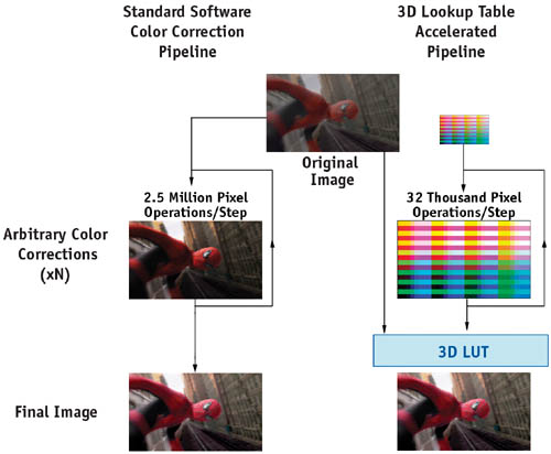
Figure 24-6 Comparing Color-Correction Pipelines
We summarize our 3D LUT acceleration framework as follows:
- Generate (and cache) the 3D lattice as a 2D image, preferably in the same byte order as the GPU will expect in step 3.
- Apply arbitrary color correction to this lattice image (using a standard color-correction pipeline), treating the 3D lattice image as a proxy for the final color correction you wish to apply.
- Load both the high-resolution image and the 3D texture to the GPU.
- Draw source imagery using the fragment shader in Listing 24-1.
The potential speedups of this optimization are enormous. In our experience, we can often substitute the full image processing (2048x1556 pixels) with a lattice of only 32x32x32 (256x128 pixels). Assuming the application of the LUT has low overhead (which is definitely the case on modern hardware), this corresponds to a speedup of approximately 100 times! Furthermore, in video playback applications, the LUT transform does not need to be recomputed, and can be applied to each subsequent frame at essentially no cost.
24.2.4 Extending 3D LUTs for Use with High-Dynamic-Range Imagery
High-dynamic-range (HDR) data breaks one of our primary assumptions in the use of lookup tables, that of the limited input domain.
Clamping
We cannot create a tabular form of a color transform if we do not first define the bounds of the table. We thus must choose minimum and maximum values to represent in the lookup table. The subtlety is that if we define a maximum that is too low, then we will unnecessarily clamp our data. However, if we define a maximum that is too high, then we will needlessly throw away table precision. (Which means our LUT sampling will be insufficient to re-create all but the smoothest of color transforms.)
Defining color-space minimums of less than zero is occasionally useful, particularly when color renderings can result in out-of-gamut colors, or when filters with negative lobes have been applied. However, for the majority of users, the transform floor can be safely pinned to zero.
Choosing a color-space ceiling is not too difficult, as HDR spaces are rarely completely unconstrained. [3] More often than not, even color spaces defined as "high-dynamic" (having pixel values greater than one) often have enforceable ceilings dictated for other reasons. For example, in linear color spaces directly derived from the Cineon (log) negative specification (Kennel and Snider 1993), the maximum defined value is approximately 13.5. [4] Even in color space not tied directly to film densities, allowing for completely unconstrained highlights wreaks havoc with filter kernel sizes. In the majority of practical compositing situations, a reasonable maximum does exist—just know your data sets and use your best judgment.
Nonuniformly Sampled Lattices
Once we have picked a ceiling and a floor for the range we wish to sample, we still have the issue of sample distribution. Say we have set our ceiling at a pixel value of 100.0. Dividing this into equally sampled regions for a 32x32x32 LUT yields a cell size of about 3. Assuming a reasonable exposure transform, almost all perceptually significant results are going to be compressed into the few lowest cells, wasting the majority of our data set.
We thus want to place our samples in the most visually significant locations, which typically occur closer to the dark end of the gamut. We achieve this effect by wrapping our 3D lookup-table transform with a matched pair of 1D "shaper" LUTs, as shown in Figure 24-7. The ideal shaper LUT maps the input HDR color space to a normalized, perceptually uniform color space. [5] The 3D LUT is then applied normally (though during its computation, this 1D transform must be accounted for). Finally, the image is mapped through the inverse of the original 1D LUT, "unwrapping" the pixel data back into their original dynamic range.
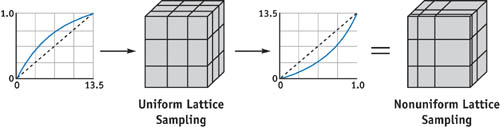
Figure 24-7 Creating a Nonuniform Lattice Sampling
24.3 Conclusion
We have presented a production-ready algorithm that allows the real-time color processing of high-resolution imagery, offering speedup of greater than 100 times on common applications. This technique is independent of both the number of color operators applied and the underlying color transform complexity. It is our hope that these ideas will enable real-time, sophisticated color corrections to become more commonplace, both in the visual effects industry as well as in consumer applications.
24.4 References
Bjorke, Kevin. 2004. "Color Controls." In GPU Gems, edited by Randima Fernando, pp. 363–373. Addison-Wesley. This chapter presents a general overview of color correction on the GPU. Also outlines the use of 1D LUTs in color correction.
Blinn, Jim. 1998. Jim Blinn's Corner: Dirty Pixels. Morgan Kaufmann. Contains an excellent discussion of quantization errors inherent in integer color spaces.
Brinkman, Ron. 1999. The Art and Science of Digital Compositing. Morgan Kaufmann. A primer on basic compositing and image processing.
Chuang, Yung-Yu, Brian Curless, David H. Salesin, and Richard Szeliski. 2001. "A Bayesian Approach to Digital Matting." In Proceedings of IEEE Computer Vision and Pattern Recognition (CVPR 2001) 2, pp. 264–271.
ICC. 2004. International Color Consortium Specification ICC.1:2004-04. Available online at http://www.color.org . ICC profiles leverage 3D LUTs to encode acquisition and display device performance characteristics.
Kang, Henry. 1997. Color Technology for Electronic Imaging Devices. SPIE. Chapter 4 contains information on 3D LUTs in color applications, including additional interpolation types.
Kennel, Glenn, and David Snider. 1993. "Gray-Scale Transformations of Digital Film Data for Display, Conversion, and Film Recording." SMPTE Journal 103, pp. 1109–1119.
Larson, Greg W., and Rob A. Shakespeare. 1998. Rendering with Radiance: The Art and Science of Lighting Visualization. Morgan Kaufmann.
Toomer, G. J. 1996. "Trigonometry." In Oxford Classical Dictionary, 3rd ed. Oxford.
Wyszecki, G., and W. S. Stiles. 1982. Color Science: Concepts and Methods, Quantitative Data and Formulae, 2nd ed. Wiley.
Copyright
Many of the designations used by manufacturers and sellers to distinguish their products are claimed as trademarks. Where those designations appear in this book, and Addison-Wesley was aware of a trademark claim, the designations have been printed with initial capital letters or in all capitals.
The authors and publisher have taken care in the preparation of this book, but make no expressed or implied warranty of any kind and assume no responsibility for errors or omissions. No liability is assumed for incidental or consequential damages in connection with or arising out of the use of the information or programs contained herein.
NVIDIA makes no warranty or representation that the techniques described herein are free from any Intellectual Property claims. The reader assumes all risk of any such claims based on his or her use of these techniques.
The publisher offers excellent discounts on this book when ordered in quantity for bulk purchases or special sales, which may include electronic versions and/or custom covers and content particular to your business, training goals, marketing focus, and branding interests. For more information, please contact:
U.S. Corporate and Government Sales
(800) 382-3419
corpsales@pearsontechgroup.com
For sales outside of the U.S., please contact:
International Sales
international@pearsoned.com
Visit Addison-Wesley on the Web: www.awprofessional.com
Library of Congress Cataloging-in-Publication Data
GPU gems 2 : programming techniques for high-performance graphics and general-purpose
computation / edited by Matt Pharr ; Randima Fernando, series editor.
p. cm.
Includes bibliographical references and index.
ISBN 0-321-33559-7 (hardcover : alk. paper)
1. Computer graphics. 2. Real-time programming. I. Pharr, Matt. II. Fernando, Randima.
T385.G688 2005
006.66—dc22
2004030181
GeForce™ and NVIDIA Quadro® are trademarks or registered trademarks of NVIDIA Corporation.
Nalu, Timbury, and Clear Sailing images © 2004 NVIDIA Corporation.
mental images and mental ray are trademarks or registered trademarks of mental images, GmbH.
Copyright © 2005 by NVIDIA Corporation.
All rights reserved. No part of this publication may be reproduced, stored in a retrieval system, or transmitted, in any form, or by any means, electronic, mechanical, photocopying, recording, or otherwise, without the prior consent of the publisher. Printed in the United States of America. Published simultaneously in Canada.
For information on obtaining permission for use of material from this work, please submit a written request to:
Pearson Education, Inc.
Rights and Contracts Department
One Lake Street
Upper Saddle River, NJ 07458
Text printed in the United States on recycled paper at Quebecor World Taunton in Taunton, Massachusetts.
Second printing, April 2005
Dedication
To everyone striving to make today's best computer graphics look primitive tomorrow
- Copyright
- Inside Back Cover
- Inside Front Cover
- Part I: Geometric Complexity
-
- Chapter 1. Toward Photorealism in Virtual Botany
- Chapter 2. Terrain Rendering Using GPU-Based Geometry Clipmaps
- Chapter 3. Inside Geometry Instancing
- Chapter 4. Segment Buffering
- Chapter 5. Optimizing Resource Management with Multistreaming
- Chapter 6. Hardware Occlusion Queries Made Useful
- Chapter 7. Adaptive Tessellation of Subdivision Surfaces with Displacement Mapping
- Chapter 8. Per-Pixel Displacement Mapping with Distance Functions
- Part II: Shading, Lighting, and Shadows
-
- Chapter 9. Deferred Shading in S.T.A.L.K.E.R.
- Chapter 10. Real-Time Computation of Dynamic Irradiance Environment Maps
- Chapter 11. Approximate Bidirectional Texture Functions
- Chapter 12. Tile-Based Texture Mapping
- Chapter 13. Implementing the mental images Phenomena Renderer on the GPU
- Chapter 14. Dynamic Ambient Occlusion and Indirect Lighting
- Chapter 15. Blueprint Rendering and "Sketchy Drawings"
- Chapter 16. Accurate Atmospheric Scattering
- Chapter 17. Efficient Soft-Edged Shadows Using Pixel Shader Branching
- Chapter 18. Using Vertex Texture Displacement for Realistic Water Rendering
- Chapter 19. Generic Refraction Simulation
- Part III: High-Quality Rendering
-
- Chapter 20. Fast Third-Order Texture Filtering
- Chapter 21. High-Quality Antialiased Rasterization
- Chapter 22. Fast Prefiltered Lines
- Chapter 23. Hair Animation and Rendering in the Nalu Demo
- Chapter 24. Using Lookup Tables to Accelerate Color Transformations
- Chapter 25. GPU Image Processing in Apple's Motion
- Chapter 26. Implementing Improved Perlin Noise
- Chapter 27. Advanced High-Quality Filtering
- Chapter 28. Mipmap-Level Measurement
- Part IV: General-Purpose Computation on GPUS: A Primer
-
- Chapter 29. Streaming Architectures and Technology Trends
- Chapter 30. The GeForce 6 Series GPU Architecture
- Chapter 31. Mapping Computational Concepts to GPUs
- Chapter 32. Taking the Plunge into GPU Computing
- Chapter 33. Implementing Efficient Parallel Data Structures on GPUs
- Chapter 34. GPU Flow-Control Idioms
- Chapter 35. GPU Program Optimization
- Chapter 36. Stream Reduction Operations for GPGPU Applications
- Part V: Image-Oriented Computing
-
- Chapter 37. Octree Textures on the GPU
- Chapter 38. High-Quality Global Illumination Rendering Using Rasterization
- Chapter 39. Global Illumination Using Progressive Refinement Radiosity
- Chapter 40. Computer Vision on the GPU
- Chapter 41. Deferred Filtering: Rendering from Difficult Data Formats
- Chapter 42. Conservative Rasterization
- Part VI: Simulation and Numerical Algorithms
-
- Chapter 43. GPU Computing for Protein Structure Prediction
- Chapter 44. A GPU Framework for Solving Systems of Linear Equations
- Chapter 45. Options Pricing on the GPU
- Chapter 46. Improved GPU Sorting
- Chapter 47. Flow Simulation with Complex Boundaries
- Chapter 48. Medical Image Reconstruction with the FFT