GPU Gems 2

GPU Gems 2 is now available, right here, online. You can purchase a beautifully printed version of this book, and others in the series, at a 30% discount courtesy of InformIT and Addison-Wesley.

The CD content, including demos and content, is available on the web and for download.

Chapter 20. Fast Third-Order Texture Filtering

Christian Sigg
ETH Zurich

Markus Hadwiger
VRVis Research Center

Current programmable graphics hardware makes it possible to implement general convolution filters in fragment shaders for high-quality texture filtering, such as cubic filters (Bjorke 2004). However, several shortcomings are usually associated with these approaches: the need to perform many texture lookups and the inability to antialias lookups with mipmaps, in particular. We address these issues in this chapter for filtering with a cubic B-spline kernel and its first and second derivatives in one, two, and three dimensions.

The major performance bottleneck of higher-order filters is the large number of input texture samples that are required, which are usually obtained via repeated nearest-neighbor sampling of the input texture. To reduce the number of input samples, we perform cubic filtering building on linear texture fetches, which reduces the number of texture accesses considerably, especially for 2D and 3D filtering. Specifically, we are able to evaluate a tricubic filter with 64 summands using just eight trilinear texture fetches.

Approaches that perform custom filtering in the fragment shader depend on knowledge of the input texture resolution, which usually prevents correct filtering of mipmapped textures. We describe a general approach for adapting a higher-order filtering scheme to mipmapped textures.

Often, high-quality derivative reconstruction is required in addition to value reconstruction, for example, in volume rendering. We extend our basic filtering method to reconstruction of continuous first-order and second-order derivatives. A powerful application of these filters is on-the-fly computation of implicit surface curvature with tricubic B-splines, which have been applied to offline high-quality volume rendering, including nonphotorealistic styles (Kindlmann et al. 2003).

20.1 Higher-Order Filtering

Both OpenGL and Direct3D provide two different types of texture filtering: nearest-neighbor sampling and linear filtering, corresponding to zeroth and first-order filter schemes. Both types are natively supported by all GPUs. However, higher-order filtering modes often lead to superior image quality. Moreover, higher-order schemes are necessary to compute continuous derivatives of texture data.

We show how to implement efficient third-order texture filtering on current programmable graphics hardware. The following discussion primarily considers the one-dimensional case, but it extends directly to higher dimensions.

To reconstruct a texture with a cubic filter at a texture coordinate x, as shown in Figure 20-1a, we have to evaluate the convolution sum

Equation 1

of four weighted neighboring texels f_i• The weights w_i (x) depend on the filter kernel used. Although there are many types of filters, we restrict ourselves to B-spline filters in this chapter. If the corresponding smoothing of the data is not desired, the method can also be adapted to interpolating filters such as Catmull-Rom splines.

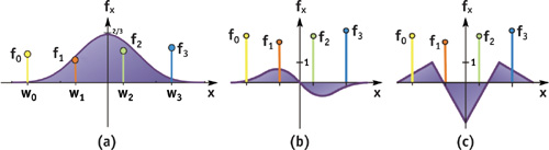
Figure 20-1 The Cubic B-Spline and Its Derivatives

Note that cubic B-spline filtering is a natural extension of standard nearest-neighbor sampling and linear filtering, which are zeroth and first-degree B-spline filters. The degree of the filter is directly connected to the smoothness of the filtered data. Smooth data becomes especially important when we want to compute derivatives. For volume rendering, where derivatives are needed for shading, it has become common practice to store precomputed gradients along with the data. Although this leads to a continuous approximation of first-order derivatives, it uses four times more texture memory, which is often constrained in volume-rendering applications. Moreover, this approach becomes impractical for second-order derivatives because of the large storage overhead. On the other hand, on-the-fly cubic B-spline filtering yields continuous first-order and second-order derivatives without any storage overhead.

20.2 Fast Recursive Cubic Convolution

We now present an optimized evaluation of the convolution sum that has been tuned for the fundamental performance characteristics of graphics hardware, where linear texture filtering is evaluated using fast special-purpose units. Hence, a single linear texture fetch is much faster than two nearest-neighbor fetches, although both operations access the same number of texel values. When evaluating the convolution sum, we would like to benefit from this extra performance.

The key idea is to rewrite Equation 1 as a sum of weighted linear interpolations between every other pair of function samples. These linear interpolations can then be carried out using linear texture filtering, which computes convex combinations denoted in the following as

Equation 2

where i = x is the integer part and = x - i is the fractional part of x. Building on such a convex combination, we can rewrite a general linear combination a x f_i + b x f_i+ ₁ with general a and b as

Equation 3

as long as the convex combination property 0 b/(a + b) 1 is fulfilled. Thus, rather than perform two texture lookups at f_i and f_i+ ₁ and a linear interpolation, we can do a single lookup at i + b/(a + b) and just multiply by (a + b).

The combination property is exactly the case when a and b have the same sign and are not both zero. The weights of Equation 1 with a cubic B-spline do meet this property, and therefore we can rewrite the entire convolution sum:

Equation 4

introducing new functions g ₀(x), g ₁(x), h ₀(x), and h ₁(x) as follows:

Equation 5

Using this scheme, the 1D convolution sum can be evaluated using two linear texture fetches plus one linear interpolation in the fragment program, which is faster than a straightforward implementation using four nearest-neighbor fetches. But most important, this scheme works especially well in higher dimensions; and for filtering in two and three dimensions, the number of texture fetches is reduced considerably, leading to much higher performance.

The filter weights w_i (x) for cubic B-splines are periodic in the interval x [0, 1]: w_i (x) = w_i (), where = x - x is the fractional part of x. Specifically,

Equation 6

As a result, the functions g_i (x) and h_i (x) are also periodic in the interval x [0, 1] and can therefore be stored in a 1D lookup texture.

We now discuss some implementation details, which include (1) transforming texture coordinates between lookup and color texture and (2) computing the weighted sum of the texture fetch results. The Cg code of the fragment program for one-dimensional cubic filtering is shown in Listing 20-1. The schematic is shown in Figure 20-2.

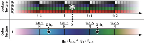
Figure 20-2 Cubic Filtering of a One-Dimensional Texture

Example 20-1. Cubic B-Spline Filtering of a One-Dimensional Texture

 float4 bspline_1d_fp( float coord_source : TEXCOORD0,    uniform sampler1D tex_source,  // source texture    uniform sampler1D tex_hg,      // filter offsets and weights      uniform float e_x,             // source texel size    uniform float size_source      // source texture size  ) : COLOR  {    // calc filter texture coordinates where [0,1] is a single texel      // (can be done in vertex program instead)    float coord_hg = coord_source * size_source – 0.5f;      // fetch offsets and weights from filter texture    float3 hg_x = tex1D( tex_hg, coord_hg ).xyz;      // determine linear sampling coordinates      float coord_source1 = coord_source + hg_x.x * e_x;    float coord_source0 = coord_source - hg_x.y * e_x;      // fetch two linearly interpolated inputs    float4 tex_source0 = tex1D( tex_source, coord_source0 );    float4 tex_source1 = tex1D( tex_source, coord_source1 );      // weight linear samples      tex_source0 = lerp( tex_source0, tex_source1, tex_hg_x.z );      return tex_source0;  }

As mentioned before, the functions g_i (x) and h_i (x) are stored in a lookup texture (called tex_hg in the listing) to reduce the amount of operations in the fragment program. In practice, a 16-bit texture of 128 samples is sufficient. Note that the functions are periodic in the sample positions of the input texture. Therefore, we apply a linear transformation to the texture coordinate and use a texture wrap parameter of GL_REPEAT for the lookup texture. In Listing 20-1, this linear transformation is incorporated into the fragment program for clarity. However, we would normally use a separate texture coordinate computed in the vertex shader.

After fetching the offsets and weights from the lookup texture, we compute the texture coordinate for the two linear texture fetches from the source color texture. Note that we need to scale the offset by the inverse of the texture resolution, which is stored in a constant-register shader parameter.

The rest of the program carries out the two color fetches and computes their weighted sum. Note that B-splines fulfill the partition of unity w_i (x) = 1, and so do the two weights g ₀(x) + g ₁(x) = 1. Therefore, we do not need to actually store g ₁(x) in addition to g ₀(x) in this case, and the final weighting is again a convex combination carried out with a single lerp() instruction.

The fragment shader parameters of Listing 20-1 would be initialized as follows for a 1D source texture with 256 texels:

 e_x = float( 1/256.0f );  size_source = float( 256.0f );

The e_x parameter corresponds to the size of a single source texel in texture coordinates, which is needed to scale the offsets fetched from the filter texture to match the resolution of the source texture. The size_source parameter simply stores the size of the source texture, which is needed to compute filter texture from source texture coordinates so that the size of the entire filter texture corresponds to a single texel of the source texture.

We now extend this cubic filtering method to higher dimensions, which is straightforward due to the separability of tensor-product B-splines. Actually, our optimization works even better in higher dimensions. Using bilinear or trilinear texture lookups, we can combine 4 or 8 summands into one weighted convex combination. Therefore, we are able to evaluate a tricubic filter with 64 summands using just eight trilinear texture fetches.

The offset and weight functions for multidimensional filtering can be computed independently for each dimension using Equation 5. In our implementation, this leads to multiple fetches from the same one-dimensional lookup texture. The final weights and offsets are then computed in the fragment program using

Equation 7

where the index k denotes the axis and are the basis vectors. Listing 20-2 shows an implementation that minimizes the number of dependent texture reads by computing all texture coordinates at once.

Example 20-2. Bicubic B-Spline Filtering

 float4 bspline_2d_fp( float2 coord_source : TEXCOORD0,    uniform sampler2D tex_source,  // source texture    uniform sampler1D tex_hg,      // filter offsets and weights      uniform float2 e_x,            // texel size in x direction    uniform float2 e_y,            // texel size in y direction    uniform float2 size_source     // source texture size    ) : COLOR  {    // calc filter texture coordinates where [0,1] is a single texel    // (can be done in vertex program instead)    float2 coord_hg = coord_source * size_source - float2(0.5f, 0.5f);      // fetch offsets and weights from filter texture      float3 hg_x = tex1D( tex_hg, coord_hg.x ).xyz;    float3 hg_y = tex1D( tex_hg, coord_hg.y ).xyz;      // determine linear sampling coordinates    float2 coord_source10 = coord_source + hg_x.x * e_x;    float2 coord_source00 = coord_source - hg_x.y * e_x;      float2 coord_source11 = coord_source10 + hg_y.x * e_y;    float2 coord_source01 = coord_source00 + hg_y.x * e_y;    coord_source10 = coord_source10 - hg_y.y * e_y;    coord_source00 = coord_source00 - hg_y.y * e_y;      // fetch four linearly interpolated inputs      float4 tex_source00 = tex2D( tex_source, coord_source00 );    float4 tex_source10 = tex2D( tex_source, coord_source10 );    float4 tex_source01 = tex2D( tex_source, coord_source01 );    float4 tex_source11 = tex2D( tex_source, coord_source11 );      // weight along y direction      tex_source00 = lerp( tex_source00, tex_source01, hg_y.z );    tex_source10 = lerp( tex_source10, tex_source11, hg_y.z );      // weight along x direction    tex_source00 = lerp( tex_source00, tex_source10, hg_x.z );      return tex_src00;  }

The fragment shader parameters of Listing 20-2 would be initialized as follows for a 2D source texture with 256 x 128 texels:

 e_x = float2( 1/256.0f, 0.0f );  e_y = float2( 0.0f, 1/128.0f );    size_source = float2( 256.0f, 128.0f );

The particular way the source texel size is stored in the e_x and e_y parameters allows us to compute the coordinates of all four source samples with a minimal number of instructions, because in this way we can avoid applying offsets along the x axis for all four samples, as shown in Listing 20-2. In three dimensions, the same approach makes it possible to compute all eight source coordinates with only 14 multiply-add instructions.

Filtering in three dimensions is a straightforward extension of Listing 20-2.

20.3 Mipmapping

For mipmapped textures, we run into the problem that the offset and scale operations of texture coordinates that correspond to the input texture resolution cannot be done with uniform fragment shader constants as shown in Listings 20-1 and 20-2. When a texture is mipmapped, the appropriate texture resolution changes on a per-fragment basis (for GL_*_MIPMAP_NEAREST filtering) or is even a linear interpolation between two adjacent texture resolutions (for GL_*_MIPMAP_LINEAR filtering).

In this chapter, we describe only the case of GL_*_MIPMAP_NEAREST filtering in detail. However, GL_*_MIPMAP_LINEAR filtering can also be handled with a slightly extended approach that filters both contributing mipmap levels with a bicubic filter and interpolates linearly between the two in the fragment shader.

For our filtering approach, we need to know the actual mipmap level and corresponding texture resolution used for a given fragment in order to obtain correct offsets (e_x, e_y, e_z) and scale factors (size_source). However, on current architectures, it is not possible to query the mipmap level in the fragment shader. We therefore use a workaround that stores mipmap information in what we call a meta-mipmap. The meta-mipmap is an additional mipmap that in each level stores the same information in all texels, such as the resolution of this level. A similar approach can be used to simulate derivative instructions in the fragment shader (Pharr 2004).

We use a floating-point RGB texture for the meta-mipmap, as follows:

 // RGB meta-mipmap information for each texel of a given mipmap_level  metatexel = float3( 1/level_width, 1/level_height, mipmap_level );

The following code fragment shows how the size_source and e_x, e_y scales and offsets in Listings 20-1 and 20-2 (where they were uniform parameters) can then be substituted by a correct per-fragment adaptation to the actual mipmap level used by the hardware for the current fragment:

 // fetch meta-mipmap information  float3 meta = tex2D( tex_meta, coord_source ).xyz;    // compute scales from offsets so we do not need to store them  float2 size_source = float2( 1.0f/meta.x, 1.0f/meta.y );    // filter texture coordinates  // where [0,1] is a single texel of the source texture    // (cannot be done in the vertex program anymore)  float2 coord_hg = coord_source * size_source - 0.5f;    // adjust neighbor sample offsets  e_x *= meta.x;  e_y *= meta.y;

Now e_x and e_y are initialized to unit vectors instead of being premultiplied with the texture dimensions:

 e_x = float2( 1.0f, 0.0f );  e_y = float2( 0.0f, 1.0f );

For GL_*_MIPMAP_NEAREST filtering, we do not need the third component of the meta-mipmap (meta.z), which stores the mipmap level itself. However, to implement GL_*_MIPMAP_LINEAR filtering, we also need the interpolation weight between the two contributing mipmap levels. This weight can then be obtained as frac(meta.z) from the third meta-mipmap component as interpolated by the hardware.

An important consideration when using a meta-mipmap is its texture memory footprint, which can be quite high when used in a straightforward manner. Theoretically, we would need a meta-mipmap for each texture size and aspect ratio that an application is using in order to get the corresponding mipmap information. However, this memory overhead can be reduced considerably.

First, we use only a single meta-mipmap that matches the highest texture resolution used in the application (called meta_baselevel_size). To get correct mipmapping information for any resolution, we strip higher resolutions of the meta-mipmap on the fly by setting the GL_TEXTURE_BASE_LEVEL texture parameter to match the resolution of the current texture (called target_size):

 glTexParameter( GL_TEXTURE_2D, GL_TEXTURE_BASE_LEVEL,                  log2( meta_baselevel_size / target_size ) );

Second, a meta-mipmap of height 1 can indeed be used for all aspect ratios and dimensions if the fragment shader profile supports the ddx() and ddy() functions for obtaining partial derivatives of texture coordinates with respect to screen coordinates. These functions, together with the variant of tex2D(), which accepts user-supplied derivatives, allow us to simulate all aspect ratios with respect to mipmap level selection even without knowing the actual mipmap level.

The texture fetch from the meta-mipmap is then performed with modified derivatives:

 // fetch and modify derivatives  // requires uniform float2 meta_adjust; see below  float2 meta_ddx = ddx( coord_source ) * meta_adjust;  float2 meta_ddy = ddy( coord_source ) * meta_adjust;    // sample meta-mipmap with modified derivatives  float3 meta = tex2D( tex_meta, coord_src, meta_ddx, meta_ddy ).xyz;

The uniform parameter meta_adjust must be set in order to adapt the actual aspect ratio of the meta-mipmap to the aspect ratio of the target texture, where cur_base_size is the actual size of the current GL_TEXTURE_BASE_LEVEL of the meta-mipmap:

 meta_adjust = float2( target_size_x/cur_base_size, target_size_y );

Because we supply modified derivatives that ultimately determine the mipmap level that the hardware will use, we effectively simulate a different aspect ratio of the meta-mipmap without requiring the corresponding storage.

In summary, the meta-mipmap texture memory footprint can be reduced to a single 1D texture with the highest texture resolution (of any axis) the application is using. This single meta-mipmap can then be used when filtering any application texture by setting the meta-mipmap's GL_TEXTURE_BASE_LEVEL and the meta_adjust uniform fragment shader parameter accordingly. Figure 20-3 shows the quality improvement using higher-order texture filtering of a 2D texture.

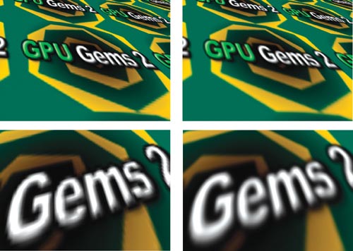
Figure 20-3 Comparing Texture-Filter Quality with Bilinear and Bicubic Reconstruction Filters

20.4 Derivative Reconstruction

In addition to reconstructing the values in a texture map, the reconstruction of its derivatives also has many applications. For example, in volume rendering, the gradient of the volume is often used as a surface normal for shading. The gradient g of a scalar field f, in this case a 3D texture, is composed of its first partial derivatives:

Equation 8

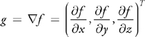
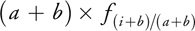
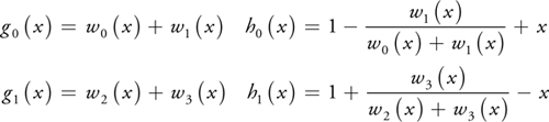
The most common method for approximating gradient information is to use a simple central differencing scheme. However, for high-quality derivatives, we can also use convolution filters and apply the scheme illustrated previously for fast evaluation on GPUs. Figure 20-4 shows the quality improvement using higher-order gradients for Phong shading of isosurfaces. To reconstruct a derivative via filtering, we convolve the original data with the derivative of the filter kernel. Figures 20-1b and 20-1c (back on page 314) illustrate the first and second derivatives of the cubic B-spline. Computing the derivative becomes very similar to reconstructing the function value, just using a different filter kernel.

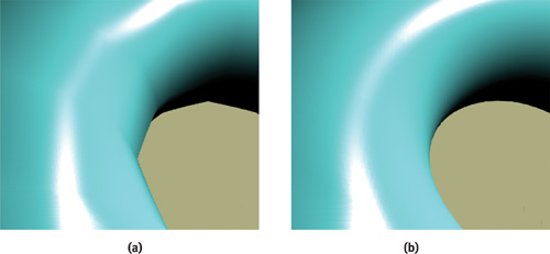
Figure 20-4 Comparing Shading Quality with Trilinear and Tricubic Reconstruction Filters

We can apply the fast filtering scheme outlined previously for derivative reconstruction with the cubic B-spline's derivative. The only difference in this case is that now all the filter kernel weights sum up to zero instead of one: w_i (x) = 0. Now, in comparison to Listing 20-1, where the two linear input samples were weighted using a single lerp(), we obtain the second weight as the negative of the first one; that is, g ₁(x) = -g ₀(x), which can be written as a single subtraction and subsequent multiplication, as shown in Listing 20-3.

Example 20-3. First-Derivative Cubic B-Spline Filtering of a One-Dimensional Texture

 // . . . unchanged from Listing 20-1      // weight linear samples    tex_source0 = ( tex_source0 - tex_source1 ) * hg_x.z;      return tex_source0;  }

To compute the gradient in higher dimensions, we obtain the corresponding filter kernels via the tensor product of a 1D derived cubic B-spline for the axis of derivation, and 1D (nonderived) cubic B-splines for the other axes.

In addition to first partial derivatives, second partial derivatives can also be computed very quickly on GPUs. All these second derivatives taken together make up the Hessian matrix H, shown here for the 3D case:

Equation 9

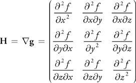
The mixed derivatives in H (the off-diagonal elements) can be computed using the fast filtering approach for first derivatives that we have just described, because the 1D filter kernels are derived only once in this case.

For the diagonal elements of H, however, the derivative of the filter kernel itself has to be taken two times. Figure 20-1c shows the second derivative of the cubic B-spline, which is a piecewise linear function. The convolution sum with this filter is very simple to evaluate. Listing 20-4 shows how to do this using three linearly interpolated input samples. In this case, no filter texture is needed, due to the simple shape of the filter. The three input samples are simply fetched at unit intervals and weighted with a vector of (1, -2, 1).

Example 20-4. Second-Derivative Cubic B-Spline Filtering of a One-Dimensional Texture

 float4 bspline_dd_1d_fp( float coord_source : TEXCOORD0,    uniform sampler1D tex_source,  // source texture    uniform float e_x,             // source texel size    ) : COLOR  {    // determine additional linear sampling coordinates    float coord_source1 = coord_source + e_x;    float coord_source0 = coord_source - e_x;      // fetch three linearly interpolated inputs    float4 tex_source0 = tex1D( tex_source, coord_source0 );    float4 tex_sourcex = tex1D( tex_source, coord_source );    float4 tex_source1 = tex1D( tex_source, coord_source1 );      // weight linear samples      tex_source0 = tex_source0 - 2 * tex_sourcex + tex_source1;      return tex_source0;  }

A very useful application of high-quality first and second derivative information is computing implicit surface curvature from volume data stored in a 3D texture. Implicit surface curvature in this case is the curvature of isosurfaces, which can easily be rendered on graphics hardware (Westermann and Ertl 1998).

Implicit curvature information can be computed directly from the gradient g and the Hessian matrix H (Kindlmann et al. 2003), for which tricubic B-spline filters yield high-quality results. Each of the required nine components (three for g and six for H, due to symmetry), requires the evaluation of a separate tricubic convolution filter, which has traditionally been extremely expensive. However, using the fast filtering scheme described in this chapter, it can actually be done in real time on current GPUs. Figure 20-5 shows images that have been generated in real time with the isosurface volume rendering demo applications that are included on the book's CD.

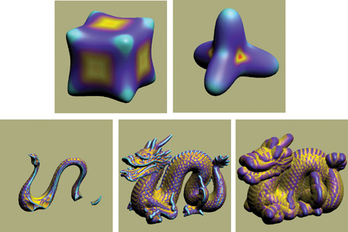
Figure 20-5 Nonphotorealistic Isosurface Rendering Using On-the-Fly Maximum Curvature Evaluation

20.5 Conclusion

This chapter has presented an efficient method for third-order texture filtering with a considerably reduced number of input texture fetches. Building on the assumption that a linear texture fetch is as fast as or not much slower than a nearest-neighbor texture fetch, we have optimized filtering with a third-order filter kernel such as a cubic B-spline to build on a small number of linear texture fetches. A cubic output sample requires 2 instead of 4 input samples, a bicubic output sample can be computed from 4 instead of 16 input samples, and tricubic filtering is possible with 8 instead of 64 fetches from the input texture. In fact, the corresponding fragment programs are more similar to "hand-coded" linear interpolation than to cubic filtering.

Another advantage of this method is that all computations that depend on the filter kernel are precomputed and stored in small 1D lookup textures. This way, the actual fragment shader can be kept independent from the filter kernel in use (Hadwiger et al. 2001). The fragment shaders for value and first-derivative reconstruction that we have shown can be used without change with a Gaussian filter of appropriate width, for example.

A disadvantage of building on linear input samples is that it may require higher precision of the input texture for high-quality results. On current GPUs, linear interpolation of 8-bit textures is also performed at a similar precision, which is not sufficient for tricubic filtering, where a single trilinearly interpolated sample contains the contribution of 8 input samples. We have used 16-bit textures in our implementation, which provides sufficient precision of the underlying linear interpolation. Many current-generation GPUs also support filtering of floating-point textures, which would provide even higher precision.

In another vein, we have used our filters for function (or derivative) reconstruction, which in OpenGL terminology is called magnification filtering. For higher-order filters to also work with texture minification, we have shown how to extend their use to mipmapped textures. An important component of this introduced here is the reduction of the memory footprint of the required additional texture information (which we call a meta-mipmap).

Finally, we have shown how our method can be used for high-quality reconstruction of first and second partial derivatives, which is especially useful for volume rendering or rendering implicit surfaces represented by a signed distance field, for example. With this method, differential surface properties such as curvature can also be computed with high quality in real time.

20.6 References

Bjorke, Kevin. 2004. "High-Quality Filtering." In GPU Gems, edited by Randima Fernando, pp. 391–415. Addison-Wesley. Gives a very nice overview of different applications for high-quality filtering with filter kernels evaluated procedurally in the fragment shader.

Hadwiger, Markus, Thomas Theußl, Helwig Hauser, and Eduard Gröller. 2001. "Hardware-Accelerated High-Quality Filtering on PC Hardware." In Proceedings of Vision, Modeling, and Visualization 2001, pp. 105–112. Stores all filter kernel information in textures and evaluates arbitrary convolution sums in multiple rendering passes without procedural computations or dependent texture lookups. Can be implemented in a single pass on today's GPUs.

Kindlmann, Gordon, Ross Whitaker, Tolga Tasdizen, and Torsten Möller. 2003. "Curvature-Based Transfer Functions for Direct Volume Rendering: Methods and Applications." In Proceedings of IEEE Visualization 2003, pp. 513–520. Shows how implicit surface curvature can be computed directly from first and second partial derivatives obtained via tricubic B-spline filtering, along with very nice applications, including nonphotorealistic rendering.

Pharr, Matt. 2004. "Fast Filter-Width Estimates with Texture Maps." In GPU Gems, edited by Randima Fernando, pp. 417–424. Addison-Wesley. Uses the concept of mipmaps that store information about the mipmap level itself in all pixels of a given mipmap level for approximating the ddx() and ddy() fragment shader instructions.

Westermann, Rüdiger, and Thomas Ertl. 1998. "Efficiently Using Graphics Hardware in Volume Rendering Applications." In Proceedings of SIGGRAPH 98, pp. 169–177. Shows how to render isosurfaces of volume data by using the hardware alpha test and back-to-front rendering. On current GPUs, using the discard() instruction and front-to-back rendering provides better performance in combination with early-z testing.

The authors would like to thank Markus Gross and Katja Bühler for their valuable contributions and Henning Scharsach for his implementation of a GPU ray caster. The first author has been supported by Schlumberger Cambridge Research, and the second author has been supported by the Kplus program of the Austrian government.

Copyright

Many of the designations used by manufacturers and sellers to distinguish their products are claimed as trademarks. Where those designations appear in this book, and Addison-Wesley was aware of a trademark claim, the designations have been printed with initial capital letters or in all capitals.

The authors and publisher have taken care in the preparation of this book, but make no expressed or implied warranty of any kind and assume no responsibility for errors or omissions. No liability is assumed for incidental or consequential damages in connection with or arising out of the use of the information or programs contained herein.

NVIDIA makes no warranty or representation that the techniques described herein are free from any Intellectual Property claims. The reader assumes all risk of any such claims based on his or her use of these techniques.

The publisher offers excellent discounts on this book when ordered in quantity for bulk purchases or special sales, which may include electronic versions and/or custom covers and content particular to your business, training goals, marketing focus, and branding interests. For more information, please contact:

U.S. Corporate and Government Sales
(800) 382-3419
corpsales@pearsontechgroup.com

For sales outside of the U.S., please contact:

International Sales
international@pearsoned.com

Visit Addison-Wesley on the Web: www.awprofessional.com

Library of Congress Cataloging-in-Publication Data

GPU gems 2 : programming techniques for high-performance graphics and general-purpose
computation / edited by Matt Pharr ; Randima Fernando, series editor.
p. cm.
Includes bibliographical references and index.
ISBN 0-321-33559-7 (hardcover : alk. paper)
1. Computer graphics. 2. Real-time programming. I. Pharr, Matt. II. Fernando, Randima.

T385.G688 2005
006.66—dc22
2004030181

GeForce™ and NVIDIA Quadro® are trademarks or registered trademarks of NVIDIA Corporation.

mental images and mental ray are trademarks or registered trademarks of mental images, GmbH.

All rights reserved. No part of this publication may be reproduced, stored in a retrieval system, or transmitted, in any form, or by any means, electronic, mechanical, photocopying, recording, or otherwise, without the prior consent of the publisher. Printed in the United States of America. Published simultaneously in Canada.

For information on obtaining permission for use of material from this work, please submit a written request to:

Pearson Education, Inc.
Rights and Contracts Department
One Lake Street
Upper Saddle River, NJ 07458

Text printed in the United States on recycled paper at Quebecor World Taunton in Taunton, Massachusetts.

Second printing, April 2005

Dedication

To everyone striving to make today's best computer graphics look primitive tomorrow

Part II: Shading, Lighting, and Shadows

Part III: High-Quality Rendering

Part IV: General-Purpose Computation on GPUS: A Primer

Part V: Image-Oriented Computing

Part VI: Simulation and Numerical Algorithms