GPU Gems 2

GPU Gems 2 is now available, right here, online. You can purchase a beautifully printed version of this book, and others in the series, at a 30% discount courtesy of InformIT and Addison-Wesley.

The CD content, including demos and content, is available on the web and for download.

Chapter 38. High-Quality Global Illumination Rendering Using Rasterization

Toshiya Hachisuka
The University of Tokyo

While the visual richness of images that current GPUs can render interactively continues to increase quickly, there are many important lighting effects that are not easily handled with current techniques. One important lighting effect that is difficult for GPUs is high-quality global illumination, where light that reflects off of objects in the scene that are not themselves light emitters is included in the final image. Incorporating this indirect illumination in rendered images greatly improves their visual quality; Figure 38-1 shows an indoor scene with indirect lighting and large area light sources. Like all images in this chapter, it was rendered with a GPU-based global illumination algorithm that uses rasterization hardware for efficient ray casting.

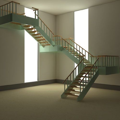
Figure 38-1 An Image Rendered with Global Illumination Accelerated by the GPU

Techniques for including these effects usually require ray tracing for high-quality results. At each pixel, a "final gather" computation is done, in which a large number of rays are cast over the hemisphere around the point, in order to sample the light arriving from many different directions. This chapter describes an approach for using the GPU's rasterization hardware to do fast ray casting for final gathering for high-quality offline rendering. In contrast to previous techniques for GPU ray tracing (for example, Purcell et al. 2002 and Carr et al. 2002), this approach is based on using the rasterization hardware in an innovative way to perform ray-object intersections, rather than on mapping classic ray-tracing algorithms to the GPU's programmable fragment processing unit. Even though our target is images of the highest quality, rather than images rendered at interactive frame rates, the enormous amounts of computational capability and bandwidth available on the GPU make it worthwhile to use for offline rendering.

38.1 Global Illumination via Rasterization

Rather than adapt various CPU-based global illumination methods to the GPU, we argue that it is more natural and efficient to derive a new global illumination algorithm that employs rasterization, because graphics hardware is based on rasterization rendering. Although many previous techniques use the GPU to perform real-time rendering with some features of global illumination—such as precomputed radiance transfer (Sloan et al. 2002)—it is also attractive to use the GPU for accelerating high-quality offline rendering. One important advantage of using rasterization in this way is that we do not need to maintain ray-tracing acceleration structures (such as uniform grids) on the GPU. This is a significant advantage, because previous GPU-based ray tracers have depended on the CPU for building these structures and were thus limited both by the CPU's processing speed as well as by the amount of memory available on the GPU for storing the complete scene description. Our technique suffers essentially from neither of these problems.

We have posted our global illumination renderer, named "Parthenon," which uses the techniques presented here, at http://www.bee-www.com/parthenon/. This application can also be found on the book's CD. Figure 38-2 shows additional images rendered by Parthenon.

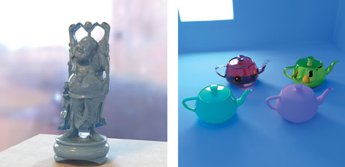
Figure 38-2 Images Rendered Using Parthenon, a GPU-Accelerated Renderer

38.2 Overview of Final Gathering

38.2.1 Two-Pass Methods

Conceptually, the easiest way to solve global illumination is to use path tracing, but this approach requires a great number of rays to obtain an image without noise. As a result, most global illumination renderers today implement a more efficient two-pass method. Two-pass methods compute a rough approximation to the global illumination in the scene as a first pass, and then in a second pass, they render the final image efficiently using the results of the first pass. Many renderers use radiosity or photon mapping for the first pass. Although the result of the first pass can be used directly in the final image, achieving sufficient quality to do so often requires more computation time than using a two-pass method (that is, we need a large number of photons to obtain a sufficiently accurate image if we use photon mapping). Figure 38-3 shows global illumination renderings of a Cornell Box using direct visualization of photon mapping and using the two-pass method. These images take nearly the same amount of computation time.

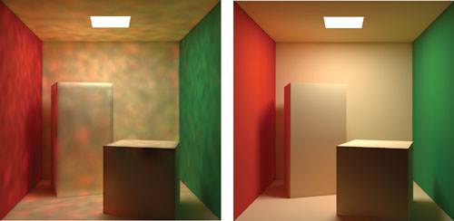
Figure 38-3 Comparing Results from Direct Use of the Photon Map and from the Two-Pass Method

Although it sounds redundant to process the same scene twice, the computational cost of a first pass is usually not very large, because it computes an approximate result. Thus, the first pass accounts for only a small part of the total rendering time. This method is the de facto standard of recent global illumination renderers because it can produce a final image with sufficient quality faster than path tracing usually can.

38.2.2 Final Gathering

There is a wide variety of ways in which the first-pass solution can be used, but the most popular method is to use it as a source of indirect illumination when evaluating a hemispherical integral via ray casting in the second pass. At each visible point, we would like to determine how much light is arriving at the point from other objects in the scene. To do so, we cast a large number of rays over the hemisphere at that point to determine which object in the scene is visible along each direction and how much light is arriving from it, as shown in Figure 38-4. This process is called final gathering. The resulting radiance (brightness) of each visible point can be computed by the following integral:

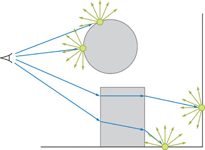
Figure 38-4 The Basic Idea of Final Gathering

This equation shows that the outgoing radiance of the specified point is the integral of the cosine-weighted reflected incident radiance according to the BRDF. We need ray casting to compute the incident radiance L_in in this integral.

38.2.3 Problems with Two-Pass Methods

In practice, the final gathering step is usually the bottleneck of the whole rendering process, because it requires a great number of ray-casting operations to achieve sufficiently accurate results for a final image. Table 38-1 shows the number of rays of each process in a typical scene.

Table 38-1. The Number of Rays for a Typical Scene

Photon Tracing	Ray Tracing from Camera	1024 Samples Final Gathering
607,002	262,144	268,435,456
15,886,408	323,212	101,261,312
368,793	379,452	253,227,008

If we assume that CPU ray tracing has a performance of 250,000 rays per second to render the Cornell Box scene in Table 38-1, the final gathering process takes about 20 minutes, whereas ray tracing from the camera takes about 1 second. For this reason, many renderers use an interpolation approach that performs final gathering on only a sparse sampling point set and interpolates the result on the rest of the points (Ward 1994). Although this approach can reduce the duration of the final gathering process, it cannot be greatly reduced if the scene generates many sampling points due to geometric complexity. Moreover, as a practical problem, it is necessary to adjust many nonintuitive parameters for the interpolation not to introduce obvious artifacts. Because we need to render the scene several times to find optimal values of the parameter, this approach may not reduce "total" rendering time so much if such trial-and-error time is included.

38.3 Final Gathering via Rasterization

Our GPU-based final gathering method calculates the hemispherical integral at all visible points, so interpolation is no longer necessary—all you need to adjust is the total number of samples! Moreover, because this method processes all visible points at the same time, we can see this rendering process progressively and terminate the computation when the resulting image achieves sufficient quality. Our method leverages the capabilities of the GPU's rasterization hardware, such that this approach is usually faster than those based on final gathering on the CPU at a sparse set of points and using interpolation.

38.3.1 Clustering of Final Gathering Rays

For each visible point, the final gathering step generates N uniformly distributed rays over the hemisphere centered around the visible point's normal vector, as shown in Figure 38-5a. Rather than choose these directions differently at every point, as most CPU-based implementations do (we call it hemispherical clustering), our method chooses the direction of each generated ray from a predetermined set of N fixed directions (we call it parallel clustering). This set of directions can be thought of as a discretization of all the directions over the unit sphere. Consider now all of the rays generated for all of the visible points. If you group the rays that have the same predetermined direction into N subsets, each subset will consist of rays with different origins but the same direction (Figure 38-5b).

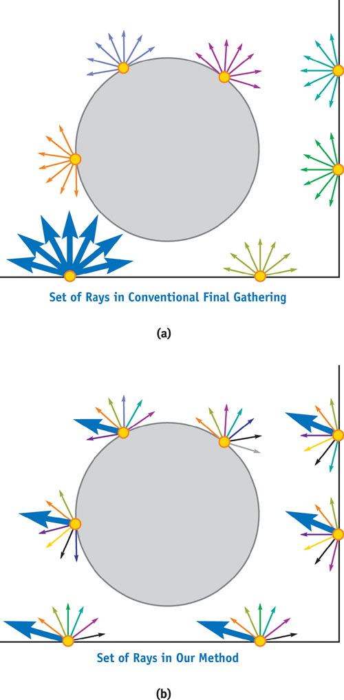
Figure 38-5 Two Different Clusterings of Final Gathering Rays

Our method makes direct use of parallel clustering of rays: instead of tracing the rays associated with each visible point separately, we choose one of the N predetermined directions at a time, and we effectively trace all of the rays with this direction simultaneously using rasterization. This rasterization is performed via a parallel projection of the scene along the current direction. The currently selected direction is called the global ray direction. The concept of the global ray direction itself has been previously proposed by Szirmay-Kalos and Purgathofer (1998). Although we can use the hemicube method (Cohen et al. 1993) with hemispherical clustering of rays, this is a very time-consuming approach, because we need to rasterize the scene on the order of the number of pixels. Note that our method only requires rasterization on the order of the number of global ray directions (that is, the number of final gathering samples). Usually, the number of pixels is orders of magnitude larger than the number of final gathering samples, so the proposed method is very efficient.

38.3.2 Ray Casting as Multiple Parallel Projection

The key to considering final gathering as multiple parallel projections is the concept of a depth layer. Depth layers are subsets of the geometry in a scene, based on the number of intersections along a certain direction, starting from outside the scene, as shown in Figure 38-6. For example, a ray arrives at the second depth layer for rays shot in the opposite of the global ray direction after intersecting the first depth layer. Thus, after choosing a particular global ray direction, all we have to do is obtain the nearest point along the global ray direction starting from a particular position by using depth layers. Because the nearest point exists on the nearest depth layer starting from a visible point, if we can fetch the nearest depth layer based on the position of the parallel projection of the visible point (see Figure 38-7), this process is equivalent to ray casting.

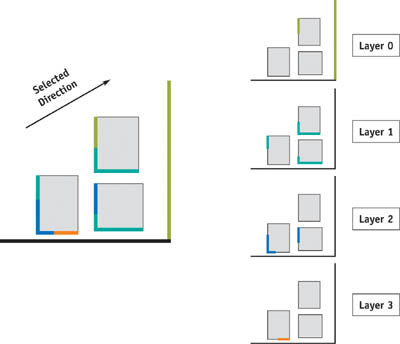
Figure 38-6 Depth Layers of a Simple Scene Along a Particular Direction

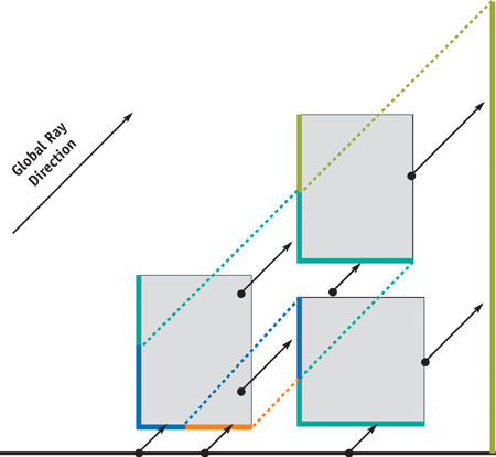
Figure 38-7 Parallel Multiple Ray Casts as a Parallel Projection

To obtain each depth layer by using the GPU, we use the multipass rendering method called depth peeling (Everitt 2001). Although this method was invented to sort geometry for correct alpha blending, it is essentially based on the concept of depth layers. With depth peeling, the rendering of the scene is first performed as usual. The next rendering pass ignores fragments with the same depth as those rendered in the first pass, so that the fragments that have the next larger depth value than those in the first depth layer are stored in the frame buffer. As a result, we can extract all depth layers in order by repeating this process.

38.4 Implementation Details

Now that we have the tools for performing final gathering on the GPU by rasterization, we explain the details of the implementation of our algorithm. The following steps summarize the method.

Store the position and normal at each visible point to visible point buffer A.
Initialize "depth" buffer B and buffer C to maximum distance.
Clear sampled depth layer buffer D to zero.
Sample one global ray direction by uniform sampling.
Read buffer D at the position of parallel projection of the visible point in buffer A, and store the result into buffer E if this point is in front of the visible point along the selected global ray direction.
Render the scene geometry, including the data from the first pass, into buffer B (for depth value) and buffer D (for color) using parallel projection by selected global ray direction, with reversed depth test (that is, render the farthest point of the mesh). If the fragment of the point has larger depth value than buffer C, then it is culled.
Copy buffer B into buffer C.
Return to step 5 until the number of the rendered fragments becomes 0 at step 6.
Accumulate buffer E into indirect illumination buffer.
Return to step 2 until the number of samplings becomes sufficient.

38.4.1 Initialization

At first, we need to store the data of visible points to the floating-point texture, to start the final gathering process. The simplest way to do this is to render the position and the normal of vertices by storing this data as texture coordinates. We describe later the details of generating this data for global illumination rendering. Note that these visible points are arbitrary (that is, each visible point's data is independent of the others). Therefore, we can process not only points visible from the camera, but also any set of data such as texels of light maps, the baked colors of vertices, and so on. In addition to the data of visible points, we also need to sample global ray direction and store this vector into a pixel shader constant. For the successive depth peeling process, we fill the two "depth" buffers B and C (these buffers are not depth stencil buffers!) to maximum distance.

38.4.2 Depth Peeling

Because depth peeling needs two depth buffers, we use two textures as depth buffers. We extract depth layers from farthest to nearest along the global ray direction. Therefore, at first, each visible point samples the farthest intersection point, whereas we need the nearest intersection point. We extract depth layers in turn and sample the depth layer if the sampled point is in front of the visible point along the selected direction. By iterating this process, each visible point finally gets its nearest intersection point, as shown in Figure 38-8.

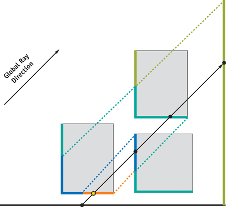
Figure 38-8 Obtaining the Nearest Intersection Point

To extract each depth layer, we render the scene depth value with the reversed depth test (that is, the farthest fragment is rendered) to "depth" buffer B and cull the resulting fragment if its distance is farther than the corresponding value in "depth" buffer C. The data of this fragment is stored into buffer D for sampling of the depth layer. Then buffer B is copied to buffer C for the next iteration. This iteration extracts each depth layer to buffer D.

38.4.3 Sampling

We can sample the nearest intersection points by depth peeling, as just described. For each iteration, we project visible points by parallel projection and read the buffer D if the point is in front of the projected visible point. The resulting sampled point is stored into buffer E. Note that buffer E will be overwritten if the sampled point is nearer than the stored point in buffer E. Finally, buffer E stores the nearest intersection point from the visible point position with the global ray direction.

If we clear buffer D to the corresponding color from the environment map at step 3, we can simultaneously sample direct illumination by image-based lighting. (However, this sampling method is limited to uniform sampling because the distribution of indirect illumination for each point is different. Therefore, we usually use a separate direct illumination step with a more elaborate sampling method, as described later.) Note that the number of fragments does not need to be completely zero at the conditional branch of step 8 of our algorithm. If you are willing to allow some rendering errors, the number of fragments used as the ending condition can be some value (such as 2 percent of the total number of fragments) rather than zero; setting this value larger than zero can reduce the number of iterations and improve performance.

38.4.4 Performance

Because the presented algorithm is completely different from ray-traced final gathering on the CPU, comparing the two is difficult. However, current performance is nearly the same as an interpolation method (such as irradiance gradients) on the CPU. Note that our method does final gathering on all pixels. Compared to doing final gathering on all pixels using the CPU, our GPU-rasterization-based method is much faster. Its performance typically approaches several million rays cast per second. That matches or beats the best performance of highly optimized CPU ray tracing (Wald et al. 2003). Note that this high CPU performance depends on all rays being coherent, which is not the case when final gathering is used.

38.5 A Global Illumination Renderer on the GPU

Given the ability to do final gathering quickly with the GPU, we now discuss the practical implementation of a global illumination renderer on the GPU using our technique. The actual implementation of any global illumination renderer is quite complex, so to simplify the explanation here, we limit the discussion to Lambertian materials, and to such renderer features as soft shadows, interreflection, antialiasing, depth-of-field effects, and image-based lighting.

38.5.1 The First Pass

As already explained, a rough global illumination calculation is performed in the first pass. Here we use grid photon mapping on the CPU because this method is somewhat faster than ordinary photon mapping. Grid photon mapping accumulates photons into a grid data structure and uses a constant-time, nearest-neighbor query (that is, a query of the grid) at the cost of precision. After constructing this grid representation of the photon map, we compute the irradiance values as vertex colors in a finely tessellated mesh. Note that you can also use any data structure to store irradiance, such as light maps or volume textures (for example, Greger et al. 1998). We don't explain the implementation details here because you can use any kind of global illumination technique on the CPU or the GPU. The important thing is to generate the irradiance distribution quickly, and the resulting data should be accessed easily and instantly by the GPU's rasterization in the successive GPU final gathering step. Therefore, for example, it may not be efficient to use photon mapping on the GPU (Purcell et al. 2003), because implementations of this approach so far have all estimated the irradiance on the fly. Note that, as mentioned in Section 38.2, we can get a rough global illumination result by rendering this mesh with irradiance data.

38.5.2 Generating Visible Points Data

Before beginning the illumination process, we have to prepare the position, normal vector, and color of visible points. To do so, we simply render the scene from the camera and write out this data to floating-point buffers using a fragment shader. Using multiple render target functionality for this process is useful, if it is available.

These buffers can be used directly during the illumination process, or you can use accumulation buffer techniques to increase the quality of the final image. For example, antialiasing can be performed by jittering the near plane of the view frustum on a subpixel basis when generating the visible point set (Haeberli and Akeley 1990). It is better to use quasi-Monte Carlo methods or stratified sampling for jittering. In rasterization rendering, we can use a great number of samples to perform antialiasing, because it is done simply by changing the perspective projection matrix.

Similarly, to achieve depth-of-field effects, the position of the camera can also be jittered. The amount of jittering in this case is varied with the aperture/form of the lens or the position of the focal plane. Because the image resulting from this technique is equivalent to a ray-traced depth-of-field effect, we don't have any of the problems that are associated with image-based depth of field, such as edge bleeding. If you would like to combine this effect with antialiasing, all you have to do is jitter both the camera position and the near plane.

38.5.3 The Second Pass

Because the proposed final gathering computes indirect illumination only, we have to compute direct illumination independently and sum these results later. When computing direct illumination, we use typical real-time shadowing techniques, such as shadow mapping and stencil shadows. In our system, area lights are simulated by using many point light source samples and taking the average of these contributions.

To perform image-based lighting, we consider each environment light as a collection of parallel light sources. Note that uniform sampling is not helpful in almost all image-based lighting, because the use of high dynamic range usually produces very large variation in illumination. Therefore, one should use an importance-based sampling method, such as the one presented in Agarwal et al. 2003.

In both cases, note that the calculation of direct illumination using graphics hardware is very fast compared to CPU-based ray tracing. As a result, we can very quickly obtain an image with a much larger number of samples compared to using ray-traced shadows.

For indirect illumination, we perform the final gathering method on the GPU, as described earlier, by using the result of the first pass as vertex colors. We use the position, normal vector, and color buffers as a visible points set, and we use mesh data with irradiance values at the vertices as a mesh for rendering. To obtain a final image, we add the indirect illumination to the direct illumination.

38.5.4 Additional Solutions

We now discuss some additional implementation problems, along with examples of how they can be solved.

Aliasing

Because the final gathering method is based on rasterization using parallel projection to a limited resolution buffer, there is an aliasing problem similar to that of shadow mapping. This aliasing often results in leaks of indirect illumination. An example of this aliasing is shown in Figure 38-9. This problem is exactly the same as that of shadow mapping; therefore, as in shadow mapping, we can address aliasing to some degree by using perspective shadow mapping (Stamminger and Dretakkis 2002) or some other elaborate method. We don't go into the implementation details here because they exceed the range of this chapter.

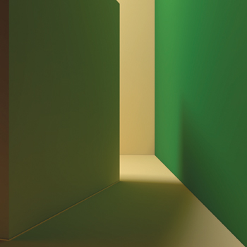
Figure 38-9 Close-up of an Aliasing Artifact

Flickering and Popping

Although using photon mapping for the first pass is an efficient global illumination method, in a scene with a moving object, flickering may occur due to the randomness of photon shooting. To solve this problem, we can also use the final gathering method described in this chapter. Note that the final gathering method generates the radiance distribution reflected N times, given the radiance distribution reflected N - 1 times. This observation implies that you can solve the global illumination problem itself using the following algorithm, which is illustrated in Figure 38-10.

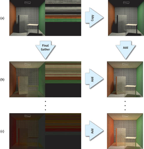
Figure 38-10 Computing Global Illumination Using Final Gathering

First, a light source is sampled using a quasi-Monte Carlo sampling, and the resulting illumination data (irradiance distribution reflected zero times), consisting of direct illumination only, is recorded into a buffer of vertex data using the direct illumination technique. Next, we perform final gathering with global ray direction at the triangle vertices using the quasi-Monte Carlo method and this illumination data, and we accumulate the results into another buffer of vertex data. As a result, we get reflected "0 + 1" time global illumination data (that is, direct illumination and indirect illumination data after reflecting one time) using the GPU-based final gathering method. To compute all of the indirect illumination, we simply iterate this process, generating illumination data reflected n + 1 times, one after another, and then accumulate this data into a buffer. Note that each step doesn't need a large number of samples, as final rendering does. By using this precomputation method, flickering and popping are suppressed, because the sampling direction (that is, the global ray direction) does not change in time when we use a quasi-Monte Carlo method.

38.6 Conclusion

In this chapter we have demonstrated how to perform global illumination rendering using rasterization on the GPU. The resulting algorithm can render high-quality images efficiently. Moreover, because the proposed final gathering method is performed on all points, any set of points (such as texels of light maps or baked colors of vertices) can be easily processed. The final gather step itself is simply a hemispherical integral calculation by ray casting, so you can also use the proposed method to perform any calculation that needs this integral value (such as form factor calculation or precomputation of radiance transfer). Our method does not currently run at interactive rates on modern GPUs, but it greatly accelerates offline rendering compared to a CPU implementation of equivalent algorithms.

38.7 References

Agarwal, S., R. Ramamoorthi, S. Belongie, and H. W. Jensen. 2003. "Structured Importance Sampling of Environment Maps." ACM Transactions on Graphics 22(3), pp. 605–612.

Carr, N. A., J. D. Hall, and J. C. Hart. 2002. "The Ray Engine." In Proceedings of the SIGGRAPH/Eurographics Workshop on Graphics Hardware 2002, pp. 37–46.

Cohen, M., and J. Wallace. 1993. Radiosity and Realistic Image Synthesis. Morgan Kaufmann.

Everitt, C. 2001. "Interactive Order-Independent Transparency." NVIDIA technical report. Available online at http://developer.nvidia.com/object/Interactive_Order_Transparency.html

Greger, G., P. Shirley, P. M. Hubbard, and D. P. Greenberg. 1998. "The Irradiance Volume." IEEE Computer Graphics and Applications (18)2, pp. 32–43.

Haeberli, P., and K. Akeley. 1990. "The Accumulation Buffer: Hardware Support for High-Quality Rendering." In Computer Graphics (Proceedings of SIGGRAPH 90) 24(4), pp. 309–318.

Purcell, T. J., I. Buck, W. R. Mark, and P. Hanrahan. 2002. "Ray Tracing on Programmable Graphics Hardware." ACM Transactions on Graphics (Proceedings of SIGGRAPH 2002) 21(3), pp. 703–712.

Purcell, T. J., C. Donner, M. Cammarano, H.-W. Jensen, and P. Hanrahan. 2003. "Photon Mapping on Programmable Graphics Hardware." In Proceedings of the SIGGRAPH/Eurographics Workshop on Graphics Hardware 2003, pp. 41–50.

Sloan, P-P., J. Kautz, and J. Snyder. 2002. "Precomputed Radiance Transfer for Real-Time Rendering in Dynamic, Low-Frequency Lighting Environments." ACM Transactions on Graphics (Proceedings of SIGGRAPH 2002) 21(3), pp. 527–536.

Stamminger, M., and G. Drettakis. 2002. "Perspective Shadow Maps." ACM Transactions on Graphics (Proceedings of SIGGRAPH 2002) 21(3), pp. 557–562.

Szirmay-Kalos, L., and W. Purgathofer. 1998. "Global Ray-Bundle Tracing with Hardware Acceleration." In Proceedings of the 9th Eurographics Workshop on Rendering, Vienna.

Wald, I., T. J. Purcell, J. Schmittler, C. Benthin, and P. Slusallek. 2003. "Realtime Ray Tracing and Its Use for Interactive Global Illumination." In Eurographics State of the Art Reports 2003.

Ward, G. 1994. "The RADIANCE Lighting Simulation and Rendering System." Computer Graphics, pp. 459–472.

Copyright

Many of the designations used by manufacturers and sellers to distinguish their products are claimed as trademarks. Where those designations appear in this book, and Addison-Wesley was aware of a trademark claim, the designations have been printed with initial capital letters or in all capitals.

The authors and publisher have taken care in the preparation of this book, but make no expressed or implied warranty of any kind and assume no responsibility for errors or omissions. No liability is assumed for incidental or consequential damages in connection with or arising out of the use of the information or programs contained herein.

NVIDIA makes no warranty or representation that the techniques described herein are free from any Intellectual Property claims. The reader assumes all risk of any such claims based on his or her use of these techniques.

The publisher offers excellent discounts on this book when ordered in quantity for bulk purchases or special sales, which may include electronic versions and/or custom covers and content particular to your business, training goals, marketing focus, and branding interests. For more information, please contact:

U.S. Corporate and Government Sales
(800) 382-3419
corpsales@pearsontechgroup.com

For sales outside of the U.S., please contact:

International Sales
international@pearsoned.com

Visit Addison-Wesley on the Web: www.awprofessional.com

Library of Congress Cataloging-in-Publication Data

GPU gems 2 : programming techniques for high-performance graphics and general-purpose
computation / edited by Matt Pharr ; Randima Fernando, series editor.
p. cm.
Includes bibliographical references and index.
ISBN 0-321-33559-7 (hardcover : alk. paper)
1. Computer graphics. 2. Real-time programming. I. Pharr, Matt. II. Fernando, Randima.

T385.G688 2005
006.66—dc22
2004030181

GeForce™ and NVIDIA Quadro® are trademarks or registered trademarks of NVIDIA Corporation.

mental images and mental ray are trademarks or registered trademarks of mental images, GmbH.

All rights reserved. No part of this publication may be reproduced, stored in a retrieval system, or transmitted, in any form, or by any means, electronic, mechanical, photocopying, recording, or otherwise, without the prior consent of the publisher. Printed in the United States of America. Published simultaneously in Canada.

For information on obtaining permission for use of material from this work, please submit a written request to:

Pearson Education, Inc.
Rights and Contracts Department
One Lake Street
Upper Saddle River, NJ 07458

Text printed in the United States on recycled paper at Quebecor World Taunton in Taunton, Massachusetts.

Second printing, April 2005

Dedication

To everyone striving to make today's best computer graphics look primitive tomorrow

Part II: Shading, Lighting, and Shadows

Part III: High-Quality Rendering

Part IV: General-Purpose Computation on GPUS: A Primer

Part V: Image-Oriented Computing

Part VI: Simulation and Numerical Algorithms