GPU Gems 2

GPU Gems 2 is now available, right here, online. You can purchase a beautifully printed version of this book, and others in the series, at a 30% discount courtesy of InformIT and Addison-Wesley.

The CD content, including demos and content, is available on the web and for download.

Chapter 17. Efficient Soft-Edged Shadows Using Pixel Shader Branching

Yury Uralsky
NVIDIA Corporation

Rendering realistic shadows has always been a hard problem in computer graphics. Soft shadows present an even greater challenge to developers, even when real-time performance is not required. Yet shadows are important visual clues that help us to establish spatial relationships between objects in a scene. In the past, artists understood the importance of shadows and used them to their advantage to emphasize certain objects and add depth to their pictures.

Real-world shadows always appear to have a certain amount of blurriness across their edges, and never appear strictly hard. Even on a bright, sunny day, when shadows are the sharpest, this is a noticeable effect. Even the sun, being a huge distance away from the Earth, can't be considered a point light source. Additionally, atmospheric scattering diffuses incoming light, blurring shadows from sunlight even more.

Recent advances in graphics hardware functionality and performance finally enable us to achieve real-time speeds when rendering soft shadows. This chapter discusses a method for rendering a high-quality approximation to real soft shadows at interactive frame rates. The method is based on adaptively taking multiple shadow-map samples in the fragment shader using a technique called percentage-closer filtering (PCF). With the branching capabilities of fragment shaders, this adaptive sampling approach provides increased visual quality while still maintaining high performance, compared to always taking a fixed number of samples.

17.1 Current Shadowing Techniques

The most well-known and robust techniques for rendering shadows are stencil shadow volumes and shadow maps. Both methods have their advantages and disadvantages.

Stencil shadow volumes work by classifying points on the scene surfaces with respect to frusta that encompass space where lighting is blocked by occluders. Sides of these frusta are formed by planes containing light-source position and edges in an object silhouette, as observed from the light source's point of view. The sides of the shadow volumes are rendered into a special off-screen buffer, "tagging" pixels in shadow. After that, normal scene rendering can color each pixel according to its tag value.

This method is simple and elegant, and it requires only minimal hardware support. It works well with both directional and point light sources, and it can be integrated pretty easily into any polygon-based rendering system such that every surface will be shadowed properly.

On the other hand, stencil shadow volumes depend heavily on how complex the geometry of a shadowing object is, and they burn a lot of fill rate. Most current implementations of the stencil shadow volumes algorithm require quite a bit of work on the CPU side, though that situation is likely to change in the future. Another downside of stencil shadow volumes is that the method is inherently multipass, which further restricts the polygon count of scenes with which it can be used.

Shadow maps are essentially z-buffers rendered as viewed from the light source's perspective. The entire scene is rendered into the shadow map in a separate pass. When the scene itself is rendered, the position of each pixel is transformed to light space, and then its z-value is compared to the value stored in the shadow map. The result of this comparison is then used to decide whether the current pixel is in shadow or not. Shadow mapping is an image-space algorithm, and it suffers from aliasing problems due to finite shadow-map resolution and resampling issues. Imagine we are looking at a large triangle positioned edge-on with respect to a light source such that the shadow stretches over it. As you can guess, its projection will cover only a handful of texels in the shadow map, failing to reproduce the shadow boundary with decent resolution. Another disadvantage of shadow maps is that they do not work very well for omnidirectional light sources, requiring multiple rendering passes to generate several shadow maps and cover the entire sphere of directions.

When their disadvantages can be avoided or minimized, shadow maps are great. Shadow maps are fully orthogonal to the rest of the rendering pipeline: everything that can be rendered and that can produce a z-value can be shadowed. Shadow maps scale very well as the triangle count increases, and they can even work with objects that have partially transparent textures. These properties have made this algorithm the method of choice for offline rendering.

Neither of these algorithms is able to produce shadows with soft edges "out of the box." Extensions to these algorithms exist that allow rendering of soft-edged shadows, but they rely on sampling the surface of the area light source and performing multiple shadow-resolution passes for each sample position, accumulating the results. This increases the cost of the shadows dramatically, and it produces visible color bands in the penumbrae of the shadows if the number of passes is not high enough.

However, it is possible to efficiently approximate soft shadows by modifying the original shadow-mapping algorithm. The percentage-closer filtering technique described by Reeves et al. (1987) takes a large number of shadow-map samples around the current point being shaded and filters their results to produce convincing soft shadows.

17.2 Soft Shadows with a Single Shadow Map

With PCF, instead of sampling the light source and rendering shadow maps at each sample position, we can get away with a single shadow map, sampling it several times in the area around the projected point in the shadow map, and then combining the results. This method does not produce physically correct soft shadows, but the visual effect is similar to what we see in reality.

17.2.1 Blurring Hard-Edged Shadows

Effectively, we are going to blur our hard-edged shadow so that it appears to have a softer edge. The straightforward way to implement this is to perform shadow-map comparisons several times using offset texture coordinates and then average the results. Intuitively, the amount of this offset determines how blurry the final shadow is.

Note that we cannot blur the actual contents of the shadow map, because it contains depth values. Instead, we have to blur the results of the shadow-map lookup when rendering a scene, which requires us to perform several lookups, each with a position offset slightly from the pixel's true position.

This approach resembles the traditional method for generating soft shadows by rendering multiple shadow maps. We just "rotate the problem 90 degrees" and replace expensive multiple shadow-map-generating passes with much less expensive multiple lookups into a single shadow map.

The GLSL code in Listing 17-1 demonstrates this idea.

Unfortunately, the naive approach only works well when the penumbra region is very small. Otherwise, banding artifacts become painfully obvious, as shown in Figure 17-1. When the number of shadow-map samples is small compared to the penumbra size, our "soft" shadow will look like several hard-edged shadows, superimposed over one another. To get rid of these banding artifacts, we would have to increase the number of shadow-map samples to a point where the algorithm becomes impractical due to performance problems.

Figure 17-1 A Naive Approach to Blurring Shadows

Example 17-1. Implementing a Basic Algorithm for PCF

 #define SAMPLES_COUNT 32  #define INV_SAMPLES_COUNT (1.0f / SAMPLES_COUNT)    uniform sampler2D decal;  // decal texture  uniform sampler2D spot;   // projected spotlight image  uniform sampler2DShadow shadowMap;  // shadow map    uniform float fwidth;  uniform vec2 offsets[SAMPLES_COUNT];    // these are passed down from vertex shader  varying vec4 shadowMapPos;  varying vec3 normal;  varying vec2 texCoord;    varying vec3 lightVec;  varying vec3 view;    void main(void)  {    float shadow = 0;    float fsize = shadowMapPos.w * fwidth;    vec4 smCoord = shadowMapPos;      for (int i = 0; i<SAMPLES_COUNT; i++) {      smCoord.xy = offsets[i] * fsize + shadowMapPos;      shadow += texture2DProj(shadowMap, smCoord) * INV_SAMPLES_COUNT;    }      vec3 N = normalize(normal);    vec3 L = normalize(lightVec);    vec3 V = normalize(view);      vec3 R = reflect(-V, N);      // calculate diffuse dot product      float NdotL = max(dot(N, L), 0);      // modulate lighting with the computed shadow value    vec3 color = texture2D(decal, texCoord).xyz;      gl_FragColor.xyz = (color * NdotL + pow(max(dot(R, L), 0), 64)) *                        shadow * texture2DProj(spot, shadowMapPos) +                        color * 0.1;  }

Let's find out how to implement this blurring in a more effective way without using too many shadow-map samples. To do this, we apply Monte Carlo methods, which are based on a probabilistic computation in which a number of randomly placed samples are taken of a function and averaged. In our context, that means we need to sample our shadow map randomly. This random placement of samples turns out to be a wise decision. The key point here is that the sequence of shadow-map sample locations is slightly different each time we calculate the shadowing value, so that the approximation error is different at different pixels. This effectively replaces banding with high-frequency noise, an artifact that the human visual system is trained to filter out very well. Note that the error is still there; it is just much better hidden from a human's eye.

If we carefully construct the sequence of offsets in a way that it has only a certain amount of randomness, we can get better results than if we use completely random offsets; this approach is called stratified or jittered sampling. To construct this distribution, we divide our domain into a number of subregions with equal areas, also known as strata, and randomly choose a sample location within each one. This subdivision provides even coverage of the domain, whereas each sample is still placed randomly within its cell.

If we assume that our sampling domain is a disk, stratification can be tricky. One possible solution is to stratify a square region and then warp it to a disk shape, preserving the area of the subregions. Generating a square grid of samples and then jittering it is straightforward, and for the area-preserving square-to-disk transformation, we use the following formulas:

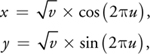
where u, v [0..1] and represent the jittered sample location within the square domain, and x, y are the corresponding sample position within the disk domain. Figure 17-2 illustrates the process. This way, the u dimension maps to angular position and the v dimension maps to radial distance from the disk center. The square roots compensate for the change in the cells' area as we move from the disk center outward, reducing the radial size of the cells.

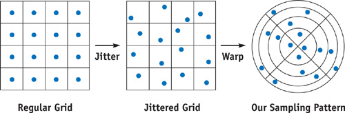
Figure 17-2 Jittering a Regular Grid and Warping to a Disk

17.2.2 Improving Efficiency

To achieve good shadow quality, we still need to take quite a few samples. We may need to take as many as 64 samples to have good-looking shadows with smooth penumbrae.

Think about it: we need to sample the shadow map 64 times per pixel. This places significant pressure on texture memory bandwidth and shader processing.

Fortunately, most real-world shadows don't have a large penumbra region. The penumbra region is the soft part of the shadow, and it is where the most samples are needed. The other pixels are either completely in the shadow or completely out of the shadow, and for those pixels, taking one sample would give the same result as taking thousands of them.

Branching Like a Tree

Of course, we want to skip unnecessary computations for as many pixels as possible. But how do we know which pixels are in penumbrae and which are not? As you can guess, implementing this would require us to make decisions at the fragment level.

GeForce 6 Series GPUs finally enable true dynamic branching in fragment programs. This essentially means that now large blocks of code that do not need to be executed can be skipped completely, saving substantial computation.

Ideally, branch instructions would never have any overhead, and using them to skip code would only increase performance. Unfortunately, this is not the case. Modern GPUs have highly parallel, deeply pipelined architectures, calculating many pixels in concert. Pipelining allows GPUs to achieve high levels of performance, and parallelization is also natural for computer graphics, because many pixels perform similar computations. The consequence of using pipelining and parallel execution is that at any given time, a GPU processes several thousand pixels, but all of them run the same computations.

What does this have to do with branching, you say? Well, dynamic branching essentially enables pixels to choose their own execution paths. If two pixels follow different branches in their fragment program, you can no longer process those pixels together. That way, branching hurts parallelism to a certain extent.

For this reason, you want to make sure your branching is as coherent as possible. Coherence in this context means that pixels in some local neighborhood should always follow the same branch—that way, all of them can be processed together. The less coherent branching is, the less benefit you'll get from skipping code with branching.

Predict and Forecast

Now let's try to predict how much benefit we can expect from branching. Basically, we need to detect whether a pixel is in the penumbra and decide how many shadow-map samples it needs. If we could come up with an inexpensive "estimator" function that would tell us whether we need more samples for the current pixel, we could use it as our branch condition.

It is impossible to find out something about the shadow map at a given pixel without actually sampling the shadow map. It also seems obvious that one sample is not enough to determine if the current pixel is only partly in shadow. So, we need a way to determine that with a small number of samples.

Therefore, we take a small number of shadow-map samples and compare them. If they all happen to have the same value (that is, all of them are either ones or zeroes), then it is very likely that the rest of the samples within the same region will have the same value. This works because most shadows are "well behaved": changes between lit and shadowed areas are pretty infrequent compared to penumbra size. The smaller the number of samples we take to try to figure this out, the bigger the benefit we gain from branching.

The next question is how to place our estimation samples to make the penumbra prediction as precise as possible. If these samples have fixed locations within the sampling domain, once again we will suffer from banding. But we know how to deal with banding: jitter the samples again!

As it turns out, the best we can do is distribute the jittered samples in a circle near the edge of the disk, where they are most likely to catch the transition from light to shadow, as shown in Figure 17-3.

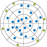
Figure 17-3 Estimation Samples (Shown in Green)

Of course, this placement of samples will fail to catch penumbrae for some pixels. But thanks to jittering, the next pixel will have a slightly different placement of estimation samples and will probably get it correct. That way, we again dissipate prediction error in high-frequency noise across adjacent pixels.

17.2.3 Implementation Details

For the shadow map itself, we use a depth texture and a "compare" texture application mode that are standard in OpenGL 1.4. Note that using floating-point formats for shadow maps is usually overkill and adds the unnecessary burden of having to manually perform comparisons in the fragment shader. As an additional benefit, NVIDIA hardware supports free four-sample bilinear percentage-closer filtering of depth textures, which helps to smooth out the penumbrae even more.

The bulk of our algorithm deals with jittered sampling. Because generating jittered offsets is a nontrivial task, it is best to precompute them and store them in a texture (jitter map).

To avoid the color-banding issue, pixels that are near each other need to use different sets of jittering offsets. It is not a problem if the offsets repeat due to tiling of the jitter map, as long as the noise frequency is high enough to keep the effect from being noticeable.

The most natural way to implement this is to use a 3D texture to store the jittered offsets. We store unique sequences of jittered offsets in "columns" of texels along the r texture dimension, and we tile the texture in screen space along the s and t dimensions. The texture extent in the s and t dimensions determines the size of the region where sequences are different, and its size in the r dimension depends on the maximum number of samples we intend to take. Conveniently for us, GLSL provides a built-in variable, gl_FragCoord, that contains current pixel position in screen space. This is exactly what we need to address this 3D texture in the s and t dimensions.

Because our offsets are two-dimensional and texels can have up to four channels, we can employ another optimization to reduce storage requirements for this 3D texture. We store a pair of offsets per texel, with the first offset occupying the r and g components and the second one sitting in the b and a components of the texel. This way, the "depth" of our texture in texels is half the number of shadow-map samples we take per pixel. As an additional bonus, we save some amount of texture memory bandwidth, because we have to look up the texture only once for every two shadow-map samples.

Our offsets are stored in normalized form: if we distribute our samples within a disk with a radius of 1, then the center-relative offsets are always in the range [-1..1]. In a fragment program, we scale each offset by a blurriness factor to control how soft our shadows appear. Offsets don't need to be high precision, so we can get away with the signed four-component, 8-bit-per-component format for this texture.

Because our estimation samples need to be jittered too, we can use some of the offsets stored in the 3D texture for them. These should be located on the outer rings of the sampling disk. We fill our 3D texture in such a way that estimation sample offsets start at r = 0 within each column, with the rest of the offsets following. This simplifies addressing in the fragment program a bit.

To better understand the construction process for the jitter map, look at the function create_jitter_lookup() in the source code included on the accompanying CD.

Performance Notes

Shadow maps have another well-known problem related to sampling and precision. This problem is commonly called "shadow acne" and appears as shadow "leakage" on the lit side of the object, similar to z-fighting. It is usually avoided by rendering the object's back faces to the shadow map instead of its front faces. This moves the problem to the triangles facing away from the light source, which is not noticeable because those triangles are not lit by that light source and have the same intensity as shadowed surfaces.

This trick has certain performance implications with our soft shadow algorithm. Though not visible, the "acne" will have a significant impact on the branching coherence. To remedy this, we modulate our penumbra estimation result with the function (dot(N, L) <= 0 ? 0 : 1). That is, if a pixel happens to belong to the shadowed side of the object, the function will resolve to 0, effectively invalidating potentially incorrect penumbra estimation and forcing it to return a "completely in shadow" result.

Another possible improvement is to use midpoint shadow maps instead of regular shadow maps. Midpoint shadow maps work by storing an averaged depth between front faces and back faces, as viewed from the light source. When shadowing objects are closed and have reasonable thickness, this reduces shadow-aliasing artifacts as well, at the expense of more complex shadow-map construction.

The GLSL fragment shader code in Listing 17-2 illustrates the adaptive sampling approach described in this chapter.

Example 17-2. Implementing Adaptive Sampling for PCF of Shadow Maps

 #define SAMPLES_COUNT 64  #define SAMPLES_COUNT_DIV_2 32  #define INV_SAMPLES_COUNT (1.0f / SAMPLES_COUNT)    uniform sampler2D decal;   // decal texture  uniform sampler3D jitter;  // jitter map    uniform sampler2D spot;    // projected spotlight image  uniform sampler2DShadow shadowMap;  // shadow map    uniform float fwidth;  uniform vec2 jxyscale;      // these are passed down from vertex shader  varying vec4 shadowMapPos;  varying vec3 normal;  varying vec2 texCoord;  varying vec3 lightVec;  varying vec3 view;      void main(void)  {    float shadow = 0;    float fsize = shadowMapPos.w * fwidth;    vec3 jcoord = vec3(gl_FragCoord.xy * jxyscale, 0);    vec4 smCoord = shadowMapPos;      // take cheap "test" samples first      for (int i = 0; i<4; i++) {      vec4 offset = texture3D(jitter, jcoord);      jcoord.z += 1.0f / SAMPLES_COUNT_DIV_2;        smCoord.xy = offset.xy * fsize + shadowMapPos;      shadow += texture2DProj(shadowMap, smCoord) / 8;        smCoord.xy = offset.zw * fsize + shadowMapPos;      shadow += texture2DProj(shadowMap, smCoord) / 8;    }    vec3 N = normalize(normal);  vec3 L = normalize(lightVec);  vec3 V = normalize(view);    vec3 R = reflect(-V, N);      // calculate diffuse dot product  float NdotL = max(dot(N, L), 0);    // if all the test samples are either zeroes or ones, or diffuse dot  // product is zero, we skip expensive shadow-map filtering  if ((shadow - 1) * shadow * NdotL != 0) {    // most likely, we are in the penumbra      shadow *= 1.0f / 8; // adjust running total      // refine our shadow estimate    for (int i = 0; i<SAMPLES_COUNT_DIV_2 - 4; i++) {      vec4 offset = texture3D(jitter, jcoord);      jcoord.z += 1.0f / SAMPLES_COUNT_DIV_2;        smCoord.xy = offset.xy * fsize + shadowMapPos;      shadow += texture2DProj(shadowMap, smCoord)* INV_SAMPLES_COUNT;        smCoord.xy = offset.zw * fsize + shadowMapPos;      shadow += texture2DProj(shadowMap, smCoord)* INV_SAMPLES_COUNT;    }  }    // all done Ð modulate lighting with the computed shadow value  vec3 color = texture2D(decal, texCoord).xyz;    gl_FragColor.xyz = (color * NdotL + pow(max(dot(R, L), 0), 64)) *                      shadow * texture2DProj(spot, shadowMapPos) +                      color * 0.1;  }

17.3 Conclusion

We have described an efficient method for rendering soft-edged shadows in real time based on percentage-closer filtering in a fragment shader. Figure 17-4 shows sample results. This method is fully orthogonal with respect to other rendering techniques; for example, the stencil buffer can still be used for additional effects. Because most of the work is performed on the GPU, this method will demonstrate higher performance as new, more powerful GPU architectures become available.

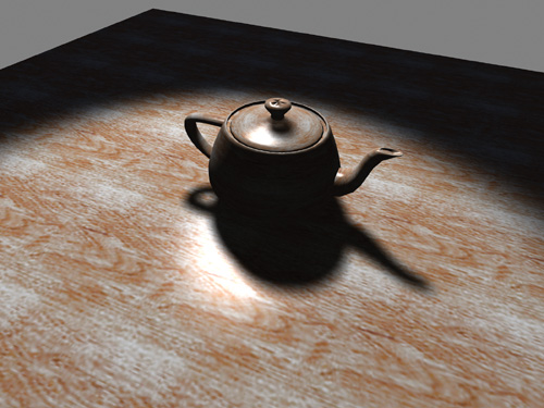
Figure 17-4 Realistic Soft-Edged Shadows in Real Time

Note that the approach described here may not work very well with unusual shadow-map projections such as perspective shadow maps. In such cases, more work is necessary to adjust the size of the penumbra on a per-pixel basis.

If used carefully, branching can provide significant performance benefits by allowing the GPU to skip unnecessary computations on a per-fragment basis. On a GeForce 6800 GT GPU, our test implementation of adaptive shadow-map sampling showed more than twice the improvement in frame rate compared to the regular shadow-map sampling. The key point for achieving high performance with branching is to keep it as coherent as possible. This will become even more important for future hardware architectures, from which we can expect even more parallelism and deeper pipelining.

17.4 References

Akenine-Möller, Tomas, and Ulf Assarsson. 2002. "Approximate Soft Shadows on Arbitrary Surfaces Using Penumbra Wedges." In Thirteenth Eurographics Workshop on Rendering, pp. 297–306.

Assarsson, Ulf, Michael Dougherty, Michael Mounier, and Tomas Akenine-Möller. 2003. "An Optimized Soft Shadow Volume Algorithm with Real-Time Performance." In Proceedings of the SIGGRAPH/Eurographics Workshop on Graphics Hardware 2003, pp. 33–40.

Brabec, Stefan, and Hans-Peter Seidel. 2002. "Single Sample Soft Shadows Using Depth Maps." In Proceedings of Graphics Interface 2002, pp. 219–228.

Cook, Robert L. 1986. "Stochastic Sampling in Computer Graphics." ACM Transactions on Graphics 5(1), pp. 51–72.

Kirsch, Florian, and Jurgen Dollner. 2003. "Real-Time Soft Shadows Using a Single Light Sample." WSCG 11(1), pp. 255–262.

Reeves, William T., David H. Salesin, and Robert L. Cook. 1987. "Rendering Antialiased Shadows with Depth Maps." Computer Graphics 21(4), pp. 283–291.

Copyright

Many of the designations used by manufacturers and sellers to distinguish their products are claimed as trademarks. Where those designations appear in this book, and Addison-Wesley was aware of a trademark claim, the designations have been printed with initial capital letters or in all capitals.

The authors and publisher have taken care in the preparation of this book, but make no expressed or implied warranty of any kind and assume no responsibility for errors or omissions. No liability is assumed for incidental or consequential damages in connection with or arising out of the use of the information or programs contained herein.

NVIDIA makes no warranty or representation that the techniques described herein are free from any Intellectual Property claims. The reader assumes all risk of any such claims based on his or her use of these techniques.

The publisher offers excellent discounts on this book when ordered in quantity for bulk purchases or special sales, which may include electronic versions and/or custom covers and content particular to your business, training goals, marketing focus, and branding interests. For more information, please contact:

U.S. Corporate and Government Sales
(800) 382-3419
corpsales@pearsontechgroup.com

For sales outside of the U.S., please contact:

International Sales
international@pearsoned.com

Visit Addison-Wesley on the Web: www.awprofessional.com

Library of Congress Cataloging-in-Publication Data

GPU gems 2 : programming techniques for high-performance graphics and general-purpose
computation / edited by Matt Pharr ; Randima Fernando, series editor.
p. cm.
Includes bibliographical references and index.
ISBN 0-321-33559-7 (hardcover : alk. paper)
1. Computer graphics. 2. Real-time programming. I. Pharr, Matt. II. Fernando, Randima.

T385.G688 2005
006.66—dc22
2004030181

GeForce™ and NVIDIA Quadro® are trademarks or registered trademarks of NVIDIA Corporation.

mental images and mental ray are trademarks or registered trademarks of mental images, GmbH.

All rights reserved. No part of this publication may be reproduced, stored in a retrieval system, or transmitted, in any form, or by any means, electronic, mechanical, photocopying, recording, or otherwise, without the prior consent of the publisher. Printed in the United States of America. Published simultaneously in Canada.

For information on obtaining permission for use of material from this work, please submit a written request to:

Pearson Education, Inc.
Rights and Contracts Department
One Lake Street
Upper Saddle River, NJ 07458

Text printed in the United States on recycled paper at Quebecor World Taunton in Taunton, Massachusetts.

Second printing, April 2005

Dedication

To everyone striving to make today's best computer graphics look primitive tomorrow

Part II: Shading, Lighting, and Shadows

Part III: High-Quality Rendering

Part IV: General-Purpose Computation on GPUS: A Primer

Part V: Image-Oriented Computing

Part VI: Simulation and Numerical Algorithms