
GPU Gems
GPU Gems is now available, right here, online. You can purchase a beautifully printed version of this book, and others in the series, at a 30% discount courtesy of InformIT and Addison-Wesley.
The CD content, including demos and content, is available on the web and for download.
Chapter 42. Deformers
Eugene d'Eon
University of Waterloo
Three-dimensional modeling and animation packages offer a wide variety of deformation tools such as Deform by Lattice and Deform by Wave. These tools allow a small number of controls to warp an arbitrarily complex mesh. Deformers can be used to quickly perform advanced modeling operations, and their controls can be animated to provide powerful animation rigs. In most cases, offloading deformation calculations from the CPU onto the GPU is possible, allowing more advanced animation systems within real-time applications and providing more interactive modeling tools. In this chapter, we will explore how to offload deformers onto the GPU, with emphasis on the problem of computing normals.
42.1 What Is a Deformer?
A deformer is an operation that takes as input a collection of vertices and generates new coordinates for those vertices (the deformed coordinates). In addition, new normals and tangents can also be generated. If you want to deform a sphere, you pass the coordinates of all its vertices to the deformer and you get back a new set of coordinates. This task is perfectly suited for vertex programs, provided that the following requirements hold:
- No vertices or edges are created or deleted by a deformer.
- The deformed coordinates of a given vertex are in no way influenced by the other vertices being processed. (A vertex averaging/smoothing operation is not a deformer because it looks at neighboring vertices.)
- The deformer is deterministic. If any two vertices have the same input coordinates before the deformation, then they will have the same output coordinates. As well, if you deform the same mesh many times, you get the same result each time.
A very simple example would be a translation. A translation deformer takes an input coordinate and returns a translated coordinate. Examples of deformers found in Softimage|XSI, Maya, and 3ds max are Deform by Curve, Cage, Lattice, Bend, Bulge, Shear, Twist, and more. The Randomize deform in Softimage|XSI is not a deformer that meets our requirements because it is not deterministic. Our technique for normal computation could not be used to implement a randomize mesh deform.
Most deformers have controls: user-defined parameters that give the deformer some variation. In most cases, controls can be animated. A wave deformer has amplitude and phase controls. A lattice deformer has lattice control points.
42.1.1 Mathematical Definition
In the most general sense, we think of a deformer as a vector-valued function, f(x, y, z). Or if you like, a deformer is three scalar functions put into a vector:
(fx (x,y,z), fy (x,y,z), fz (x,y,z)),
where fx ,fy ,fz are the component functions of f. This function f takes the coordinates (x, y, z) of a vertex and returns the deformed coordinates of that vertex. To deform a mesh, we take each vertex, input its coordinates into f, and store the output as the new vertex coordinate. Or thinking in component form, fx gives us the new x coordinate of the vertex with original coordinates (x, y, z), fy gives the new y coordinate, and so on. The deformer function f should be defined for all real values of x, y, and z, or at least some range of such values that contains the input mesh.
Spatially dependent deformers, such as a wave, will have varied results in different coordinate spaces, so passing in object, world, or eye space coordinates to f will deform in object, world, and eye space, respectively.
Linear transformations such as rotations, scales, and translations are a simple subset of all possible deformers. They take as input a set of coordinates and output a new set of coordinates (in the form of a matrix multiplication, typically). Linear transformations are not a particularly interesting set of deformers, and we already know how to compute normals under such transformations. This definition of deformers includes a much larger set of operations on geometry.
Controls
The deform operation also depends on the controls of the deformer. Controls are parameters that affect the operation of the deformer. For example, the output of a wave deformer depends on the frequency of the wave, so technically the function f depends on a variable, say freq, as well. However, we will not write f(x, y, z, freq). Instead, we will think of freq as being a constant for a given deformation operation: it does not vary across the vertices of the mesh being deformed. Therefore, it will simply appear as a constant in at least one of the component functions of f. Likewise, for a time parameter that may be used to animate a deformer: the time parameter, t, will appear as a constant in f, because time doesn't depend on coordinates x, y, and z.
42.2 Deforming on the GPU
42.2.1 Formulating the Deformer
To facilitate normal computation, it will be useful to formulate the deformer in correspondence with our mathematical definition: in functional form. If we think of a simple translation of positive 2 units in the y axis as a deformer, then the deformer f is:
f(x,y,z) = (fx ,fy ,fz ) = (x,y + 2,z).
If we are implementing a radial wave deformer, we might have

where is the phase control parameter.
Note: fx denotes the x component function of f, not to be confused with  f/x.
f/x.
42.2.2 Writing the Vertex Program
Once we have written down the deformer in functional form, deforming the vertices in a vertex program is very straightforward. Control parameters and possibly a time parameter are passed in as uniform inputs to the program (in the constant registers). To compute the vertex positions, we simply compute f(x, y, z) and store the result in the vertex position output. We apply the model and view transformations before or after computing f, depending on whether we want to deform in object, world, or view space. We may also have additional coordinate transformations to center and orient a spatially dependent deformer with respect to the object it is deforming.
What About Normals?
When we perform a linear transformation on a mesh, such as a translation, rotation, scale, or some combination of those, we know to take the matrix representation of that transformation, M, and transform the normals by the inverse transpose of M and then renormalize. [1] But linear transformations are a small subset of all possible deformers that we might want to implement in a vertex program. In general, a wave deformer can't be written in matrix form (where some constant matrix M gives us the deformed position by computing Mv) because a wave deformer is not a linear transformation. So we have no global matrix M to take the inverse transpose of and transform our normals with. We need a new technique for transforming normals.
42.2.3 Deforming Normals
How Would We Compute Normals in Software?
Animation packages first transform all vertices in the mesh by the deformer. Once that is done, it is possible to traverse the vertices in a second pass to recompute normals based on neighboring vertices in the new, deformed mesh. We don't have that option with vertex programs. Each vertex being processed in a vertex program has no knowledge of its neighbors, and there is no second stage where we can look around and do computations.
An Approximate Numerical Technique
An estimate for the deformed normal can be achieved by deforming three points for every input vertex. We find two new points very close to the input vertex. Add a very small multiple of the tangent to the vertex coordinates to get the first point. Add a very small multiple of the binormal to the vertex coordinates to get the second. These three points define two vectors whose cross product is the original normal (up to a normalization constant). We can then deform all three of these points by the deformer, and these three deformed points will define two vectors whose cross product is approximately the deformed normal (up to a normalization constant). The closer together these three points are, the more accurate the approximation will be, although numerical accuracy problems creep in if the points are too close together. It turns out that we can do better than this, however, and so avoid the numerical difficulties and the problem of choosing the extra points to deform.
The Jacobian Matrix
If a deformer f(x, y, z) = (fx , fy , fz ) has continuous first-order partial derivatives, then we can compute a matrix for each vertex called the Jacobian matrix, J. As we know, everywhere a scalar function f(x) is smooth, it is locally approximated by a straight line (a linear function: f(x)  f'(a)(x - a) + f(a), for some real number a). Likewise, everywhere the map f(x, y, z) is smooth, f can be approximated by a linear transformation, J, plus a translation (f(x) J(a)(x - a) + f(a), for some point a, and x = (x, y, z). This follows from the generalized Taylor's theorem. The Jacobian matrix is defined as follows. Note: the Jacobian matrix is often denoted Df(x).
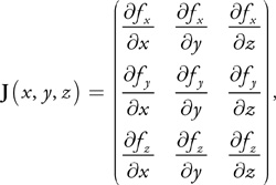
where all partial derivatives are evaluated at (x, y, z).
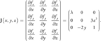
Example. Suppose we had the following deformer (where is a constant control parameter):
f(x,y,z) = (fx ,fy ,fz ) = (x,z3 ,z - y2 ).
Then the Jacobian would be:
For each position (x, y, z), we now have a linear transformation matrix J(x, y, z) that we can use to transform vectors at that position. If we had a tangent vector t at (x, y, z), then the deformed tangent would be J(x, y, z) * t (followed by a renormalize to get a unit tangent).
If we make the assumption that the vertices of the mesh are discrete samples of a smooth surface, then transforming vectors on the surface by the Jacobian matrix is valid. We can also transform normals using J(x, y, z) in two equivalent ways.
-
The inverse transpose of J(x, y, z) can be computed per vertex in the vertex program and used to transform the normal directly. If n is the input unit normal, then the deformed normal is:
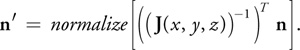
Notation: AT denotes the transpose of a matrix A.
-
If a unit tangent vector, u, is given per vertex, then we can generate a unit binormal v = n x u. We can transform the tangent and binormal to the deformed space, using the matrix J(x, y, z). Then the new, deformed normal is:

The tangent and binormal need not actually be unit length, because the final result is normalized.
Inverting 3x3 matrices is not a particularly suitable task for a vertex program, so method (2) is generally easier to implement and faster to compute. If a tangent and binormal are not given per vertex, they can be generated either on the CPU when the mesh is loaded or in the vertex program. To generate a tangent, compute two cross products, n x (0, 0, 1) and n x (0, 1, 0). Select the result with the larger magnitude. The result is a tangent vector to n. The binormal is then given by v = n x u.
Note: This technique generates discontinuous tangents and binormals across the surface and would not suffice for bump mapping and other techniques that require a continuous tangent field.
It is important to renormalize the normals, because in general normals generated with these methods will not be unit length, and most lighting equations assume unit normals.
42.3 Limitations
- Faceted meshes fail the smooth-surface assumption and will in general not give the same normals that would be achieved in software by first deforming the mesh and then recomputing faceted normals. In general, normals will vary across each face after deforming. However, in some cases this method may still create acceptable results.
- Computing the inverse of the Jacobian matrix for the purposes of transforming the normals requires that the Jacobian matrix be nonsingular at that location (that is, the determinant must be nonzero). This will be the case for most practical deformers, but it is possible to devise deformers that have ill-behaved functions that are not of maximal rank on their entire domain. At such locations, a normal cannot be computed. Both techniques described in this chapter will produce the zero vector for the deformed normal at such degenerate points. In practice, numerical errors will produce a vector very close to the zero vector, and subsequent normalize operations will generate random results.
- This method demands that the functions involved be in fact differentiable—and preferably analytically differentiable—on the domain of interest. Functions that have no known analytic derivative require using numerical derivative techniques to approximate the partial derivatives, which typically lengthen the computation greatly and are therefore highly undesirable.
- This method is limited by the length restrictions of the vertex program, especially if the Jacobian is lengthy to compute. If an object is being deformed by a series of deformers, it is probably only practical to compute the last one on the GPU. If in addition, skinning or other complex operations need to be performed in the same vertex program, then the program may have too many instructions or be too slow to compute on a large number of vertices.
42.4 Performance
As mentioned before, an alternative approximate numerical method for computing normals involves deforming three vertices for every input vertex, one very slightly along the tangent and one very slightly along the binormal. These three deformed vertices can then be used to approximate the deformed tangent and binormal, and a cross product gives the estimated deformed normal. This involves more than three times the work of deforming just the one set of vertex coordinates. In a lot of cases, computation of the Jacobian matrix can be done in fewer instructions than are required to deform two extra sets of coordinates. Expressions tend to be repeated across terms in the Jacobian, and some expressions are exactly those that were computed in computing the vertex coordinates and can be reused. This is not always the case, especially if the partial derivatives involve complicated expressions. The Jacobian method has no overhead of passing down extra coordinates and avoids most of the numerical difficulties associated with the approximate method.
Performance is a simple function of the number of instructions needed to compute the deformation. Complex deformers such as a 4x4x4 lattice deform require a lot of instructions, which will limit the amount of geometry that can be deformed in real time. In each case, the complexity of the deformer, the CPU load and GPU load of the application, and the amount of geometry to be deformed will all have to be factored in to determine if deforming on the GPU is the better solution.
42.5 Example: Wave Deformer
Here we will consider a simple circular wave with vertical displacement (in the y axis) based on radial distance from the origin in the x-z plane. In functional form we have:

where u is a wave frequency control parameter and is the wave phase parameter. We then compute the Jacobian matrix:
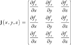
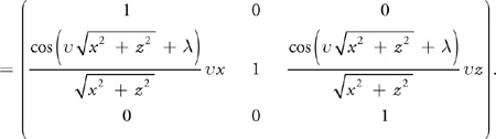
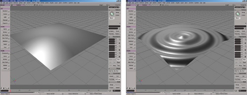
Figure 42-1 A Circular, Vertical Displacement Wave Deformer Applied to a Plane
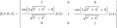
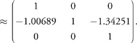
Suppose we are deforming a vertex with coordinates (3, 0, 4) and normal (0, 1, 0). Let's choose a wave frequency u = 2, and a wave phase parameter = 0. We first compute the Jacobian matrix at that location.
Next, suppose a tangent and binormal are given:
u = (-1,0,1), v = (1,0,1).
Then the transformed tangent and binormal are:
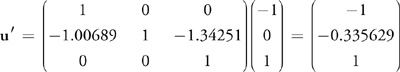
and
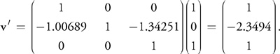
Then the deformed normal will be in the direction of:
Cross (u',v') = (2.01377,2,2.68503).
Then we normalize the last calculation to get our deformed normal:
n' = (0.515426,0.511902,0.687235).
42.6 Conclusion
We have considered a large class of mesh deformation operations and found the mathematical tools to perform such operations on the graphics hardware. The Jacobian matrix of the deformation allows us to deform normals inside the vertex program without worrying about neighboring deformed vertices. This technique is widely applicable to a number of deformation operations, keeping in mind the limitations that were observed.
Although much of this book deals with shading effects, the way that objects move and deform is just as important in creating realistic animated graphics. Currently, the quality of character animation in movies surpasses the animation in interactive graphics such as video games. This quality gap results in part from the much more sophisticated deformation techniques used in movies; most games are limited to simple skinning. We hope that over time, techniques such as those described in this chapter will help to bring the full spectrum of animation techniques to real-time productions.
Copyright
Many of the designations used by manufacturers and sellers to distinguish their products are claimed as trademarks. Where those designations appear in this book, and Addison-Wesley was aware of a trademark claim, the designations have been printed with initial capital letters or in all capitals.
The authors and publisher have taken care in the preparation of this book, but make no expressed or implied warranty of any kind and assume no responsibility for errors or omissions. No liability is assumed for incidental or consequential damages in connection with or arising out of the use of the information or programs contained herein.
The publisher offers discounts on this book when ordered in quantity for bulk purchases and special sales. For more information, please contact:
U.S. Corporate and Government Sales
(800) 382-3419
corpsales@pearsontechgroup.com
For sales outside of the U.S., please contact:
International Sales
international@pearsoned.com
Visit Addison-Wesley on the Web: www.awprofessional.com
Library of Congress Control Number: 2004100582
GeForce™ and NVIDIA Quadro® are trademarks or registered trademarks of NVIDIA Corporation.
RenderMan® is a registered trademark of Pixar Animation Studios.
"Shadow Map Antialiasing" © 2003 NVIDIA Corporation and Pixar Animation Studios.
"Cinematic Lighting" © 2003 Pixar Animation Studios.
Dawn images © 2002 NVIDIA Corporation. Vulcan images © 2003 NVIDIA Corporation.
Copyright © 2004 by NVIDIA Corporation.
All rights reserved. No part of this publication may be reproduced, stored in a retrieval system, or transmitted, in any form, or by any means, electronic, mechanical, photocopying, recording, or otherwise, without the prior consent of the publisher. Printed in the United States of America. Published simultaneously in Canada.
For information on obtaining permission for use of material from this work, please submit a written request to:
Pearson Education, Inc.
Rights and Contracts Department
One Lake Street
Upper Saddle River, NJ 07458
Text printed on recycled and acid-free paper.
5 6 7 8 9 10 QWT 09 08 07
5th Printing September 2007
- Contributors
- Copyright
- Foreword
- Part I: Natural Effects
-
- Chapter 1. Effective Water Simulation from Physical Models
- Chapter 2. Rendering Water Caustics
- Chapter 3. Skin in the "Dawn" Demo
- Chapter 4. Animation in the "Dawn" Demo
- Chapter 5. Implementing Improved Perlin Noise
- Chapter 6. Fire in the "Vulcan" Demo
- Chapter 7. Rendering Countless Blades of Waving Grass
- Chapter 8. Simulating Diffraction
- Part II: Lighting and Shadows
-
- Chapter 9. Efficient Shadow Volume Rendering
- Chapter 10. Cinematic Lighting
- Chapter 11. Shadow Map Antialiasing
- Chapter 12. Omnidirectional Shadow Mapping
- Chapter 13. Generating Soft Shadows Using Occlusion Interval Maps
- Chapter 14. Perspective Shadow Maps: Care and Feeding
- Chapter 15. Managing Visibility for Per-Pixel Lighting
- Part III: Materials
- Part IV: Image Processing
- Part V: Performance and Practicalities
-
- Chapter 28. Graphics Pipeline Performance
- Chapter 29. Efficient Occlusion Culling
- Chapter 30. The Design of FX Composer
- Chapter 31. Using FX Composer
- Chapter 32. An Introduction to Shader Interfaces
- Chapter 33. Converting Production RenderMan Shaders to Real-Time
- Chapter 34. Integrating Hardware Shading into Cinema 4D
- Chapter 35. Leveraging High-Quality Software Rendering Effects in Real-Time Applications
- Chapter 36. Integrating Shaders into Applications
- Part VI: Beyond Triangles
- Preface