GPU Gems

GPU Gems is now available, right here, online. You can purchase a beautifully printed version of this book, and others in the series, at a 30% discount courtesy of InformIT and Addison-Wesley.

The CD content, including demos and content, is available on the web and for download.

Chapter 37. A Toolkit for Computation on GPUs

Ian Buck
Stanford University

Tim Purcell
Stanford University

Traditionally the GPU has been a rendering coprocessor or, as the name implies, a graphics processing unit to the host PC. Many of the chapters in this book demonstrate how to render cool effects really fast using the GPU. But who says that the GPU is limited just to rendering? The research community has clearly demonstrated how non-graphics-related computing can be performed on the GPU, with more than a dozen papers published in the SIGGRAPH and Graphics Hardware conferences. This chapter discusses some basic approaches for performing general computation on the GPU and demonstrates how to implement some fundamental algorithms needed for many GPU-based applications.

37.1 Computing with the GPU

Why would you want to use a GPU for general computation? First: performance. Modern GPUs perform floating-point calculations much faster than today's CPUs. For example, a 3 GHz Pentium 4 can theoretically issue around 6 billion floating-point multiplies per second (6 gigaflops). However, a fragment program running on the NVIDIA GeForce FX 5900 Ultra achieves over 20 billion multiplies per second, ^[1] roughly equivalent to a 10 GHz Pentium 4. Combine this computational performance with the increased memory bandwidth available on the GPU—25.3 GB/sec peak compared to the Pentium 4's 5.96 GB/sec peak—and it's clear why the GPU outperforms the CPU. ^[2]

256-bit DDR @ 425 MHz = 425 x 2 x 32 bytes = 25.3 GB/sec

64-bit QDR @ 200 MHz = 200 x 4 x 8 bytes = 5.96 GB/sec

The second reason is load balancing. If the CPU limits the application performance, leaving the GPU with idle cycles, we can offload work to the GPU with an overall speedup in our application.

Finally, looking toward the future, GPUs are on a much faster performance growth curve than CPUs. The Pentium 4 performance over the two years leading up to June 2003 increased from 4 gigaflops to 6.3 gigaflops, or 0.65 gigaflops per year. NVIDIA GPUs, however, over only a six-month period ending with the release of the GeForce FX 5900 Ultra, increased from 8 gigaflops to 20 gigaflops, a rate of 24 gigaflops per year. In other words, GPUs have passed CPUs in performance and will continue to outpace CPUs in the future.

37.1.1 The Programming Model

As you are probably aware, there's a big difference between programming GPUs versus CPUs. We can't just change a few compiler flags and recompile. The reason is that the programming models are slightly different.

The main distinction is that the GPU is not a serial processor, but a stream processor. A serial processor, also known as a von Neumann architecture (von Neumann 1945), executes instructions sequentially, updating memory as it goes. A stream processor works in a slightly different manner—by executing a function (such as a fragment program) on a set of input records (fragments), producing a set of output records (shaded pixels) in parallel. Stream processors typically refer to this function as a kernel and to the set of records as a stream. Data is streamed into the processor, operated on via a kernel function, and output to memory, as shown in Figure 37-1. Each element passed into the processor is processed independently, without any dependencies between elements. This permits the architecture to execute the program in parallel without the need to expose the parallel units or any parallel constructs to the programmer.

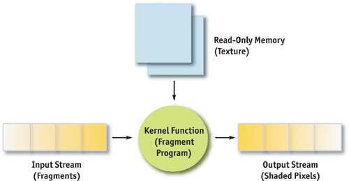
Figure 37-1 Model of a Stream Program on the GPU

As we describe in this chapter, however, these functions and records don't have to be pixels and shaders; they can just as well be arbitrary data, such as mesh points and physics equations. For example, let's say we want to implement a simple particle simulation and let the GPU perform most of the physics operations. Using floating-point textures and pixel buffers (pbuffers), we store the particle positions, velocities, and orientations. A fragment program performs the necessary calculations to compute the new position of a single particle. To compute the new position of all the particles, we simply render a large quad, where the number of fragments in the quad equals the number of particles, as shown in Figure 37-2. The texture coordinates for the quad indicate to the fragment program which stored particle it needs to process. The result stored in the pbuffer contains the new position values.

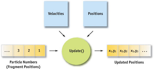
Figure 37-2 Example of a Particle System

Our example of a particle system demonstrates an obvious but useful application of the GPU for general-purpose computing. The operation of updating the positions of the particles can be generalized to the process of applying a function to an array of data. This operation—also called a map in functional programming languages—can be used for a variety of applications. Simon Green (2003) illustrated how to simulate cloth on the GPU using the same technique as our particle simulator.

37.1.2 Parallel Programming

There are some constraints on what can be mapped to the GPU. The most important is that the function must be parallelizable. Because fragment programs cannot share writable memory between different fragments, the calculations executed on each particle, mesh point, or whatever, must be computed independently of each other. Just as we cannot access the computed result of a neighboring fragment when shading, the function applied to the stream data must observe the same rule. Fortunately, most physical simulations for graphics are naturally parallel, as in the example of our particle system. Each particle does not need to know the newly computed position of its neighbor to update itself.

Using the GPU for general computation poses other challenges, which will be covered later, but the most important consideration in mapping computation to the GPU, or to most stream processors, is mandatory parallelism.

37.1.3 Advanced GPU Programming

Our simple particle system example is interesting, but what if we want to compute something more complex on the GPU? Not all applications can be implemented with a simple map operation.

The rest of this chapter describes a few basic tools you can use to implement more advanced algorithms on the GPU, with its parallel programming environment. "Reduce" provides a method to compute a single value from a set of data. "Sort and Search" provides mechanisms to build and use data structures on the GPU. Using these operations, we can perform many general-purpose computing operations that were once left to the CPU.

37.2 Reduce

In general, GPU shaders apply a function to a set of data to produce a set of results, such as applying a fragment program to shade pixels or applying a vertex shader to vertices. In either case, we pass in a set of values and get back a set of results. But what if we want only a single result from a set of values? For example, consider the problem of tone mapping. We render a high-dynamic-range scene using floating-point pbuffers and need to display the scene in the frame buffer, which has limited precision. One straightforward approach is to map the largest floating-point value to white and scale the rest of the values accordingly.

How do we get the largest value? We could read back the entire scene and let the CPU perform the computation. However, if we have to do this for every frame, the readback can seriously impede our frame rate. A better solution is to use the GPU to compute the largest value from all the pixels in the scene. In other words, use the GPU to reduce the set of floating-point pixels to a single result, the largest value.

In general, a reduction is any operation that computes a single result from a set of data. Examples include min/max, average, sum, product, or any other user-defined function. This section explains how you can use the GPU to compute reductions in just a few passes.

37.2.1 Parallel Reductions

Consider our tone-mapping example. Current graphics hardware lacks built-in features that could provide us the largest floating-point value in a pbuffer. However, we can use the programmable fragment pipeline to do a partial reduction, which will decrease the number of pixels we need to reduce.

The fragment program in Listing 37-1 outputs the largest value of four floating-point values.

Using this program, we can reduce the number of pixels by four, keeping only the larger-valued pixels. Here's how: (1) Bind the image buffer to the texture unit corresponding to the variable img and render a quad one-fourth the size of the image size (each dimension divided by two). (2) Set the texture coordinates so that each fragment of the quad corresponds to a different 2x2 rectangle in the texture. The rendered quad is one-fourth the size of the original image, keeping only the larger values. We can repeat this algorithm with the new image until we have a single floating-point value that can be read back to the CPU, as shown in Figure 37-3.

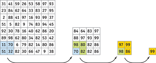
Figure 37-3 Max Reduction Performed with Multiple Passes

Example 37-1. Performing a Partial Reduction

 float main(float2 texcoord  : TEXCOORD0,    uniform samplerRECT img) : COLOR {   float a, b, c, d;   a = f1texRECT(img, texcoord);   b = f1texRECT(img, texcoord + float2(0, 1));   c = f1texRECT(img, texcoord + float2(1, 0));   d = f1texRECT(img, texcoord + float2(1, 1));   return max(max(a, b), max(c, d)); }

Performance

To perform a large reduction of a 1024x1024 image requires only ten passes, with each pass one-fourth the size of the previous pass. In general, O(log n) passes are required for performing a reduction of n ² elements. We don't necessarily need to go all the way down to one pixel for the readback. In some cases, it may be faster to read back a small square and let the CPU do the final reductions. We can also increase the number of reductions performed within the fragment program, doing more than just one reduction per pass, decreasing the total number of passes required.

37.2.2 Reduce Tidbits

Although our example is specific to tone mapping, the basic algorithm can be applied anywhere you need to do a reduction, assuming it fits within the constraints of the hardware. Obviously, we need to be able to write the reduction as a fragment program, so we are limited by the number of instructions and the size of outputs. If the GPU supports only a single four-component float output (that is, the fragment color), we cannot implement a reduction operation for a 4x4 matrix multiply (at least, not easily) that requires four four-component float outputs from the shader. Also, the situation can be more complex if the amount of data we are reducing is not a power of two in either dimension.

37.3 Sort and Search

Suppose we want to add collision detection to our particle system example for the GPU. Writing the fragment program to perform a particle-particle interaction is relatively easy. However, as more and more particles are added to the system, interacting every particle with every other particle quickly becomes expensive. The total number of passes is proportional to the number of particles in the system squared. To make matters worse, distant particles have little or no effect on a given particle. All the time spent computing interactions between distant pairs of particles is wasted frame time because these particles don't collide.

A better idea is to compute only those interactions with neighboring particles that are likely to produce collisions. One way to do this is to organize particles into a spatial data structure like a uniform grid. Neighboring particles reside in the same grid cell or group of grid cells. This method can reduce the number of particle-collision tests from n ² to a constant, based on the number of particles that fit into a grid cell and on the number of grid cells to be searched.

This section describes the two algorithms required for constructing the uniform-grid data structure for our particle system simulation: sort and search. We implement sorting as a small multipass shader, and we implement searching in a single rendering pass.

37.3.1 Bitonic Merge Sort

Sorting is a classic algorithmic problem that has inspired many different sorting algorithms. Unfortunately, most sorting algorithms are not well suited for a GPU implementation. Bitonic merge sort (Batcher 1968) is a classic parallel sorting algorithm that fits well within the constrained programming environment of the GPU.

The first step in building the uniform grid for our particle system is to sort the data into grid cells. The grid cell location for a particle is determined by dividing the scene's bounding box into cubes (grid cells). Each particle center belongs to exactly one grid cell. We can number the grid cells and then order the particles by ascending grid cell number.

Algorithm

Bitonic merge sort allows an array of n processors to sort n elements in O(log² n) steps: log n steps of up to log n stages each. Each stage performs n comparisons and swaps in parallel.

A bitonic merge sort running over an eight-element data set is shown in Figure 37-4. The arrows indicate the two elements to compare (located at the head and tail of each arrow) and the direction to swap them such that we end up with the smallest element at the tail. For example, at stage 1, step 1, we compare 4 and 8 and swap their locations since the smaller element (4) needs to be at the tail of the arrow.

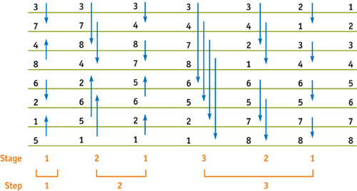
Figure 37-4 Bitonic Merge Sort over Eight Elements

Bitonic merge sort works by repeatedly grouping two sorted sequences to make a bitonic sequence, and then sorting that sequence to form a single sorted list. Recall that a bitonic sequence is one that either monotonically increases and then decreases, or decreases and then increases. Using Figure 37-4 as an example, we can see that at the end of step 1, the initial sequence has been sorted into four sublists: (3, 7), (8, 4), (2, 6), and (5, 1). These four sublists actually make up two bitonic sequences: (3, 7, 8, 4) and (2, 6, 5, 1). These two sequences get sorted in step 2. The two resulting sorted lists form the single bitonic sequence (3, 4, 7, 8, 6, 5, 2, 1). This sequence is sorted in step 3, resulting in the final sorted list.

GPU Implementation

Bitonic merge sort (and binary search, described later) requires a helper function, convert1dto2d, which simply changes 1D array addresses into 2D texture coordinates. Its implementation is straightforward, as shown in Listing 37-2.

Example 37-2. The Bitonic Merge Sort Helper Function

 float2 convert1dto2d(float coord1d, float width) {   float2 coord2d;   coord2d.y = coord1d/width;   coord2d.x = floor(frac(coord2d.y) * width);   coord2d.y = floor(coord2d.y);   return coord2d; }

Bitonic merge sort is implemented as a multipass shader. Cg code for bitonic merge sort is shown in Listing 37-3. An optimized implementation can be found on the book's CD and Web site.

The data we are sorting is stored in texture memory. Each rendering pass corresponds to a parallel comparison stage. The fragment program computes which two elements need to be compared based on the current step (stepno) and stage (stage) of the sort. The min or max value of the comparison is written out, again depending on the current stage and step of the sort. The newly generated texture is used as input to the next comparison stage. An n-element sort requires exactly (log n x (log n + 1)) ÷ 2 rendering passes.

Performance

Sorting just over a million elements (stored in a 1024x1024 texture) requires 210 rendering passes. Even the fastest graphics cards today are hard pressed to render 210 passes over a megapixel region in real time. However, sorting a smaller number of elements requires far fewer passes over a much smaller region. A data set of 4,096 elements can be sorted in only 20 milliseconds. Good CPU-based sorting routines have O(n log n) runtime asymptotics, meaning they will often be able to sort faster than the GPU. However, if the sorted data needs to live in GPU memory, the transfer time to and from the host can negate this advantage.

Example 37-3. Bitonic Merge Sort

 float BitonicSort(float2 elem2d : WPOS,                   uniform float offset,   // offset = 2^(stage - 1)     uniform float pbufwidth,                   uniform float stageno,  // stageno = 2^stage     uniform float stepno,   // stepno = 2^step     uniform samplerRECT sortedlist) : COLOR {   elem2d = floor(elem2d);   float elem1d = elem2d.y * pbufwidth + elem2d.x; 
  half csign = (fmod(elem1d, stageno) < offset) ? 1 : -1;   half cdir = (fmod(floor(elem1d/stepno), 2) == 0) ? 1 : -1; 
  float adr1d = csign * offset + elem1d;   float2 adr2d = convert1dto2d(adr1d, pbufwidth); 
  float val0 = f1texRECT(sortedlist, elem2d);   float val1 = f1texRECT(sortedlist, adr2d); 
  float cmin = (val0 < val1) ? val0 : val1;   float cmax = (val0 > val1) ? val0 : val1; 
  return (csign == cdir) ? cmin : cmax; }

37.3.2 Binary Search

Search is another classic algorithm. As mentioned during our discussion of sort, most of the algorithms for search do not work in the limited programming environment of the GPU. However, binary search is one of the most common searching algorithms, and it maps nicely onto the GPU.

With a sorted list of particles, we have almost all the data to complete our uniform-grid data structure. Although the sorted list has the particles ordered by grid cell, we have no indication of where the sublist of particles for one grid cell ends and the next list begins. We perform several sequential binary searches in parallel over our list of sorted particles to build the uniform grid. Each grid cell initiates a search for itself in the sorted list. The search returns the starting location of the particle list for every grid cell.

Algorithm

Binary search works only on a sorted list of elements. The algorithm works by looking at the middle element of a list and deciding which half of the list to examine further. This test is applied to each subsequent sublist until the sublist is of length 1. At this point, we need a final "correction" comparison to determine whether to increment the position if the value at the final position is not equal to our search value. This is an artifact of searching for the first instance of a given element, as illustrated in Figure 37-5. The algorithm requires O(log n) comparisons.

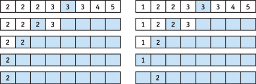
Figure 37-5 Two Binary Searches over Eight Elements for the Value 2

GPU Implementation

Binary search easily maps to a single-pass fragment program. The list of elements to be searched is stored in texture memory. A single fragment executes the entire binary search in one execution of the fragment program. The fragment program is a simple unrolled loop that iterates exactly log n + 1 times through the list. The program boils down to a sequence of dependent texture lookups. The final returned value will be either the cell searched for or the next cell's starting location. See Listing 37-4.

The Search routine, shown in Listing 37-5, simply performs the dependent texture fetch, then computes and returns the position to be examined next.

Example 37-4. Bitonic Search

 float BinarySearch(float2 elem2d : WPOS,                    uniform float stride,                    uniform float pbufwidth,                    uniform float sortbufwidth,                    uniform samplerRECT sortlist) : COLOR {   elem2d = floor(elem2d);   float elem1d = elem2d.y * pbufwidth + elem2d.x;   float curpos = stride; 
  //loop over (LOGN - 1) search passes     for(int i = 0; i < LOGN - 1; i++){     stride = floor(stride * 0.5);     curpos = Search(curpos, elem1d, stride,                      sortlist, sortbufwidth);   } 
  //log nth pass   curpos = Search(curpos, elem1d, 1.0, sortlist, sortbufwidth); 
  //cleanup pass   curpos = SearchFinal(curpos, elem1d, 1.0, sortlist, sortbufwidth); 
  return curpos; }

Example 37-5. The Search Routine

 float Search(float curpos,              float elem,              float stride,              uniform samplerRECT data,              float texw) {   float2 adr2d = convert1dto2d(curpos, texw);   float val = f1texRECT(data, adr2d);   float dir = (elem <= val) ? -1.0 : 1.0;   return dir * stride + curpos; }

Recall that after finishing the search, a final "correction" comparison is needed to possibly increment the final location. The code for SearchFinal is identical to the code for Search, except for one line:

 float dir = (elem <= val) ? 0.0 : 1.0;

Performance

Binary search is very efficient. Unlike reduce and sort, search can often be performed in a single rendering pass. A search for a single element out of more than one million sorted elements (stored in a 1024x1024 texture) requires less than a millisecond. Building a grid data structure and performing several searches in parallel consumes only a few milliseconds.

37.4 Challenges

There are some challenges that come with using current GPUs for computation—namely, limited outputs and slow readback.

37.4.1 Limited Outputs

One difficulty is the number of outputs available in the fragment program. The number of outputs supported by today's GPUs can vary from a single four-component floating-point output to four or more such outputs with the latest hardware. A limited number of outputs can restrict what we can compute in a pass. For example, if we are implementing a ray tracer where each incoming ray may produce multiple output rays (reflection, transmission, and shadow), we can easily be limited by the number of outputs supported by the GPU. This drawback should diminish as GPU technology evolves.

37.4.2 Slow Readback

Readback can be one of the biggest limitations for computation on the GPU. After computing the new particle positions, our application could use the CPU to do some challenging operation, such as collision detection with scene objects. To do this, we would read the values back from graphics card memory with the appropriate API commands. However, this requires that all of our data be sent over the AGP connection, and although modern GPUs support fast 8x AGP transfers, the readback path is only 1x AGP. ^[3] This slow transfer could wipe out any performance benefit obtained by offloading the physics calculation to the GPU. Avoiding this readback penalty provides motivation to put as much of the computation as possible on the GPU. Upcoming PCI Express–compatible motherboards should alleviate this constraint.

37.4.3 GPU vs. CPU

As we've seen in this chapter, many traditional algorithms that excel on the CPU may not map well to the GPU stream programming model. The mandatory parallelism enforced by the stream programming model, in addition to some of the constraints mentioned in this section, can force us to rethink how we solve certain problems. In some cases, the GPU is not the platform of choice for implementing an algorithm. Additionally, programming support tools such as debuggers and profilers are much more readily available on the CPU. However, we expect that many new and exciting algorithms will continue to be written for the GPU, as people learn to map their algorithms onto the stream programming model. The "Further Reading" section of this chapter includes references to some of the exciting things people are implementing on GPUs. These programs include ray tracing, photon mapping, fluid-flow solvers, cloth simulation, and global illumination calculations. Also, we expect the GPU to continue to evolve to more fully support general-purpose computation—including programmer support and tools commonly found for CPU programming.

37.5 Conclusion

This chapter demonstrates that the GPU can do quite a bit more than just render shaded pixels. We've shown four useful operations—map, reduce, sort, and search—and provided examples of how they can be used. As GPU performance continues to grow at a rapid pace, it's likely that using the GPU for general-purpose computation will become commonplace.

37.6 Further Reading

Note: www.gpgpu.org has links to several recent results and is a great repository of information for general-purpose computing on the GPU.

Batcher, Kenneth E. 1968. "Sorting Networks and Their Applications." Proceedings of AFIPS Spring Joint Computer Conference 32, pp. 307–314.

Bolz, Jeff, Ian Farmer, Eitan Grinspun, and Peter Schröder. 2003. "Sparse Matrix Solvers on the GPU: Conjugate Gradients and Multigrid." ACM Transactions on Graphics 22(3), pp. 917–924.

Carr, Nathan A., Jesse D. Hall, and John C. Hart. 2002. "The Ray Engine." Proceedings of the SIGGRAPH/Eurographics Workshop on Graphics Hardware 2002, pp. 37–46.

Carr, Nathan A., Jesse D. Hall, and John C. Hart. 2003. "GPU Algorithms for Radiosity and Subsurface Scattering." Proceedings of the SIGGRAPH/Eurographics Workshop on Graphics Hardware 2003, pp. 51–59.

Goodnight, Nolan, Rui Wang, Cliff Woolley, and Greg Humphreys. 2003. "Interactive Time-Dependent Tone Mapping Using Programmable Graphics Hardware." Eurographics Symposium on Rendering: 14th Eurographics Workshop on Rendering, pp. 26–37.

Goodnight, Nolan, Cliff Woolley, Gregory Lewin, David Luebke, and Greg Humphreys. 2003. "A Multigrid Solver for Boundary Value Problems Using Programmable Graphics Hardware." Proceedings of the SIGGRAPH/Eurographics Workshop on Graphics Hardware 2003, pp. 102–111.

Green, Simon. 2003. "Stupid OpenGL Shader Tricks." Presentation at Game Developers Conference 2003. Available online at http://developer.nvidia.com/docs/IO/8230/GDC2003_OpenGLShaderTricks.pdf

Harris, Mark J., Greg Coombe, Thorsten Scheuermann, and Anselmo Lastra. 2002. "Physically-based Visual Simulation on Graphics Hardware." Proceedings of the SIGGRAPH/Eurographics Workshop on Graphics Hardware 2002, pp. 109–118.

Harris, Mark J., William Baxter III, Thorsten Scheuermann, and Anselmo Lastra. 2003. "Simulation of Cloud Dynamics on Graphics Hardware." Proceedings of the SIGGRAPH/Eurographics Workshop on Graphics Hardware 2003, pp. 92–101.

Hillesland, Karl E., Sergey Molinov, and Radek Grzeszczuk. "Nonlinear Optimization Framework for Image-Based Modeling on Programmable Graphics Hardware." ACM Transactions on Graphics 22(3), pp. 925–934.

Krüger, Jens, and Rüdiger Westermann. 2003. "Linear Algebra Operators for GPU Implementation of Numerical Algorithms." ACM Transactions on Graphics 22(3), pp. 908–916.

Ma, Vincent C. H., and Michael D. McCool. 2002. "Low Latency Photon Mapping Using Block Hashing." Proceedings of the SIGGRAPH/Eurographics Workshop on Graphics Hardware 2002, pp. 89–99.

Moreland, Kenneth, and Edward Angel. 2003. "The FFT on a GPU." Proceedings of the SIGGRAPH/Eurographics Workshop on Graphics Hardware 2003, pp. 112–120.

Purcell, Timothy J., Ian Buck, William R. Mark, and Pat Hanrahan. 2002. "Ray Tracing on Programmable Graphics Hardware." ACM Transactions on Graphics 21(3), pp. 703–712.

Purcell, Timothy J., Craig Donner, Mike Cammarano, Henrik Wann Jensen, and Pat Hanrahan. 2003. "Photon Mapping on Programmable Graphics Hardware." Proceedings of the SIGGRAPH/Eurographics Workshop on Graphics Hardware 2003, pp. 41–50.

Sen, Pradeep, Michael Cammarano, and Pat Hanrahan. 2003. "Shadow Silhouette Maps." ACM Transactions on Graphics 22(3), pp. 521–526.

von Neumann, John. 1945. "First Draft of a Report on the EDVAC." Moore School of Electrical Engineering, University of Pennsylvania, Philadelphia. W-670-ORD-4926.

Copyright

Many of the designations used by manufacturers and sellers to distinguish their products are claimed as trademarks. Where those designations appear in this book, and Addison-Wesley was aware of a trademark claim, the designations have been printed with initial capital letters or in all capitals.

The authors and publisher have taken care in the preparation of this book, but make no expressed or implied warranty of any kind and assume no responsibility for errors or omissions. No liability is assumed for incidental or consequential damages in connection with or arising out of the use of the information or programs contained herein.

The publisher offers discounts on this book when ordered in quantity for bulk purchases and special sales. For more information, please contact:

U.S. Corporate and Government Sales
(800) 382-3419
corpsales@pearsontechgroup.com

For sales outside of the U.S., please contact:

International Sales
international@pearsoned.com

Visit Addison-Wesley on the Web: www.awprofessional.com

Library of Congress Control Number: 2004100582

GeForce™ and NVIDIA Quadro^® are trademarks or registered trademarks of NVIDIA Corporation.
RenderMan^® is a registered trademark of Pixar Animation Studios.
"Shadow Map Antialiasing" © 2003 NVIDIA Corporation and Pixar Animation Studios.
"Cinematic Lighting" © 2003 Pixar Animation Studios.
Dawn images © 2002 NVIDIA Corporation. Vulcan images © 2003 NVIDIA Corporation.

All rights reserved. No part of this publication may be reproduced, stored in a retrieval system, or transmitted, in any form, or by any means, electronic, mechanical, photocopying, recording, or otherwise, without the prior consent of the publisher. Printed in the United States of America. Published simultaneously in Canada.

For information on obtaining permission for use of material from this work, please submit a written request to:

Pearson Education, Inc.
Rights and Contracts Department
One Lake Street
Upper Saddle River, NJ 07458

Text printed on recycled and acid-free paper.

5 6 7 8 9 10 QWT 09 08 07

5th Printing September 2007

Part II: Lighting and Shadows

Part III: Materials

Part IV: Image Processing

Part V: Performance and Practicalities

Part VI: Beyond Triangles

Preface