
GPU Gems
GPU Gems is now available, right here, online. You can purchase a beautifully printed version of this book, and others in the series, at a 30% discount courtesy of InformIT and Addison-Wesley.
The CD content, including demos and content, is available on the web and for download.
Chapter 2. Rendering Water Caustics
Juan Guardado
NVIDIA
Daniel Sánchez-Crespo
Universitat Pompeu Fabra/Novarama Technology
2.1 Introduction
There is something hypnotic about the way water interacts with light: the subtle reflections and refractions, the way light bends to form dancing caustics on the bottom of the sea, and the infinitely varied look of the ocean surface. See Figure 2-1. These phenomena and their complexity have attracted many researchers from the fields of physics and, in recent years, computer graphics. Simulating and rendering realistic water is, like simulating fire, a fascinating task. It is not easy to achieve good results at interactive frame rates, and thus creative approaches must often be taken.
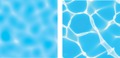
Figure 2-1 Examples of Water Caustics
Caustics result from light rays reflecting or refracting from a curved surface and hence focusing only in certain areas of the receiving surface. This chapter explains an aesthetics-driven method for rendering underwater caustics in real time. Our purely aesthetics-driven approach simply leaves realism out of consideration. The result is a scene that looks good, but may not correctly simulate the physics of the setting. As we show in this chapter, the results of our approach look remarkably realistic, and the method can be implemented easily on most graphics hardware. This simplified approach has proven very successful in many fractal-related disciplines, such as mountain and cloud rendering or tree modeling.
The purpose of this chapter is to expose a new technique for rendering real-time caustics, describing the method from its physical foundations to its implementation details. Because the technique is procedural, it yields elegantly to an implementation using a high-level shading language.
2.2 Computing Caustics
Computing underwater caustics accurately is a complex process: millions of individual photons are involved, with many interactions taking place. To simulate it properly, we must begin by shooting photons from the light source (for example, for a sea scene, the Sun). A fraction of these photons eventually collide with the ocean surface, which either reflects or refracts them. Let's forget about reflection for a moment and see how transmitted photons are refracted according to Snell's Law, which states that:
1 sin 1 = 2 sin 2,
otherwise written as:
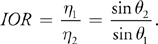
In the preceding equations, 1 and 2 are the indices of refraction for the respective materials, and 1 and 2 are the incident and refraction angles, as shown in Figure 2-2. The index of refraction, IOR, can then simply be written as the ratio of the sines of the angles of the incident and refracted rays.
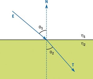
Figure 2-2 Computing Refraction
Snell's Law is not easy to code with this formulation, because it only imposes one restriction, making the computation of the refracted ray nontrivial. Assuming that the incident, transmitted, and surface normal rays are co-planar, a variety of coder-friendly formulas can be used, such as the one in Foley et al. 1996:
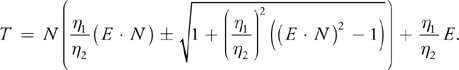
Here T is the transmitted ray, N is the surface normal, E is the incident ray, and 1, 2 are the indices of refraction.
Once bent, photons advance through the water, their intensity attenuating as they get deeper. Eventually, some of these photons will strike the ocean floor, lighting it. Due to the ocean surface's waviness, photons entering the water from different paths can end up lighting the same area of the ocean floor. Whenever this happens, we see a bright spot created by the concentration of light in a caustic, similar to the way a lens focuses light.
From a simulation standpoint, caustics are usually computed by either forward or backward ray tracing. In forward ray tracing, photons are sent from light sources and followed through the scene, accumulating their contribution over discrete areas of the ground. The problem with this approach is that many photons do not even collide with the ocean surface, and from those that actually collide with it, very few actually contribute to caustic formation. Thus, it is a brute-force method, even with some speed-ups thanks to spatial subdivision.
Backward ray tracing works in the opposite direction. It begins at the ocean floor and traces rays backward in reverse chronological order, trying to compute the sum of all incoming lighting for a given point. Ideally, this would be achieved by solving the hemispherical integral of all light coming from above the point being lit. Still, for practical reasons, the result of the integral is resolved via Monte Carlo sampling. Thus, a beam of candidate rays is sent in all directions over the hemisphere, centered at the sampling point. Those that hit other objects (such as a whale, a ship, or a stone) are discarded. On the other hand, rays that hit the ocean surface definitely came from the outside, making them good candidates. Thus, they must be refracted, using the inverse of Snell's Law. These remaining rays must be propagated in the air, to test whether each hypothetical ray actually emanated from a light source or was simply a false hypothesis. Again, only those rays that actually end up hitting a light source do contribute to the caustic, and the rest of the rays are just discarded as false hypotheses.
Both approaches are thus very costly: only a tiny portion of the computation time actually contributes to the end result. In commercial caustic processors, it is common to see ratios of useful rays versus total rays of between 1 and 5 percent.
Real-time caustics were first explored by Jos Stam (Stam 1996). Stam's approach involved computing an animated caustic texture using wave theory, so it could be used to light the ground floor. This texture was additively blended with the object's base textures, giving a nice, convincing look, as shown in Figure 2-3.
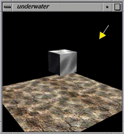
Figure 2-3 Caustics Created Using Jos Stam's Projective Caustic Texture
Another interesting approach was explored by Lasse Staff Jensen and Robert Golias in their excellent Gamasutra paper (Jensen and Golias 2001). The paper covers not only caustics, but also a complete water animation and rendering framework. The platform is based upon Fast Fourier Transforms (FFTs) for wave function modeling. On top of that, their method handles reflection, refraction, and caustics in an attempt to reach physically accurate models for each one. It is unsurprising, then, that Jensen and Golias's approach to caustics tries to model the actual process: Rays are traced from the Sun to each vertex in the wave mesh. Those rays are refracted using Snell's Law, and thus new rays are created.
2.3 Our Approach
The algorithm we use to simulate underwater caustics is just a simplification of the backward Monte Carlo ray tracing idea explained in the previous section. We make some aggressive assumptions about good candidates for caustics, and we compute only a subset of the arriving rays. Thus, the method has very low computational cost, and it produces something that, although "incorrect" physically, very closely resembles a real caustic's look and behavior. The overall effect looks very convincing, and the superior image quality given by the caustics makes it worthwhile to implement.
To begin with, we assume that we are computing caustics at noon on the Equator. This implies that the Sun is directly above us. For the sake of our algorithm, we need to compute the angle of the sky covered by the Sun disk. The Sun is between 147 and 152 million kilometers away from Earth, depending on the time of year, and its diameter is 1.42 million kilometers, which yields an angle for the Sun disk of 0.53 degrees, as shown in Figure 2-4.
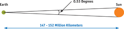
Figure 2-4 The Angle of the Sun Disk
The second assumption we make is that the ocean floor is lit by rays emanating vertically above the point of interest. The transparency of water is between 77 and 80 percent per linear meter, thus between 20 and 23 percent of incident light per meter is absorbed by the medium, which is spent heating it up. Logically, this means that caustics will be formed easily when light rays travel the shortest distance from the moment they enter the water to the moment they hit the ocean floor. Thus, caustics will be maximal for vertical rays and will not be as visible for rays entering water sideways. This is an aggressive assumption, but it is key to the success of the algorithm.
Our algorithm then works as follows. We start at the bottom of the sea, right after we have painted the ground plane. Then, a second, additive blended pass is used to render the caustic on top of that. To do so, we create a mesh with the same granularity as the wave mesh and which will be colored per-vertex with the caustic value: 0 means no lighting; 1 means a beam of very focused light hit the sea bottom. To construct this lighting, backward ray tracing is used: for each vertex of our mesh, we project it vertically until we reach the wave point located directly above it. Then, we compute the normal of the wave at that point, using finite differences. With the vector and the normal, and using Snell's Law (the index of refraction for water is 1.33), we can create secondary rays, which travel from the wave into the air. These rays are potential candidates for bringing illumination onto the ocean floor. To test them, we compute the angle between each one and the vertical. Because the Sun disk is very far away, we can simply use this angle as a measure of illumination: the closer to the vertical, the more light that comes from that direction into the ocean, as illustrated in Figure 2-5.
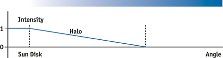
Figure 2-5 The Intensity of the Sun Disk Versus the Angle of Incidence
2.4 Implementation Using OpenGL
The initial implementation of the algorithm is just plain OpenGL code, with the only exception being the use of multipass texturing. A first pass renders the ocean floor as a regular textured quad. Then, the same floor is painted again using a fine mesh, which is lit per-vertex using our caustic generator, as shown in Figure 2-6b. For each vertex in the fine mesh, we shoot a ray vertically, collide it with the ocean surface, generate the bent ray using Snell's Law, and use that ray to perform a ray-quad test, which we use to index the texture map, as in Figure 2-6a. In the end, the operation is not very different from a planar environment mapping pass. The third and final pass renders the ocean waves using our waveform generator. These triangles will be textured with a planar environment map, so we get a nice sky reflection on them. Other effects, such as Fresnel's equation, can be implemented on top of that.
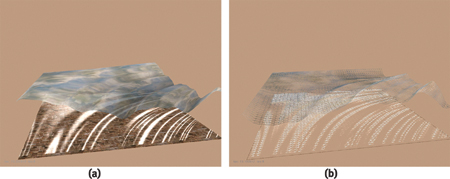
Figure 2-6 The OpenGL Implementation
The pseudocode for this technique is as follows:
- Paint the ocean floor.
- For each vertex in the fine mesh:
- Send a vertical ray.
- Collide the ray with the ocean's mesh.
- Compute the refracted ray using Snell's Law in reverse.
- Use the refracted ray to compute texture coordinates for the "Sun" map.
- Apply texture coordinates to vertices in the finer mesh.
- Render the ocean surface.
2.5 Implementation Using a High-Level Shading Language
Implementing this technique fully on the GPU gives even better visual quality and improves its performance. A high-level shading language, such as Microsoft's HLSL or NVIDIA's Cg, allows us quickly to move all these computations to the GPU, using a C-like syntax. In fact, the same wave function previously executed on the CPU in the basic OpenGL implementation was simply copied into the pixel and vertex shaders using an include file, with only minor modifications to accommodate the vector-based structures in these high-level languages.
Calculating the caustics per-pixel instead of per-vertex improves the overall visual quality and decouples the effect from geometric complexity. Two approaches were considered when porting the technique to the GPU's pixel shaders, and both use the partial derivatives of the wave function to generate a normal, unlike the original method, which relies on finite differences.
The first method takes advantage of the fact that a procedural texture can be rendered in screen space, thereby saving render time when only a small portion of the pixels are visible. Unfortunately, this also means that when a large number of pixels are visible, a lot of work is being done for each one, even though the added detail may not be appreciable. Sometimes this large amount of work can slow down the frame rate enough to be undesirable, so another method is needed to overcome this limitation.
This second method renders in texture space to a fixed-resolution render target. Although rendering in texture space has the advantage of maintaining a constant workload at every frame, the benefit of rendering only visible pixels is lost. Additionally, it becomes difficult to gauge what render target resolution most adequately suits the current scene, to the point where relying on texture filtering may introduce the tell-tale bilinear filtering cross pattern if the texel-to-pixel ratio drops too low.
We can further optimize the algorithm by observing that there is little visual difference between refracting the incoming rays using Snell's Law and simply performing environment mapping based on the distance from the water surface to the floor surface along the wave normal. See Figure 2-7. As a result, vertical rays access the center of the texture, which is bright, while angled rays produce a progressively attenuated light source. Moreover, at larger depths, the relative size of the environment map—and hence the relative size of the light source—is reduced, creating sharper caustics that can also be attenuated by distance. Note that this approach allows us to have a nonuniform ground plane, and this variable depth can easily be encoded into a scalar component of a vertex attribute.
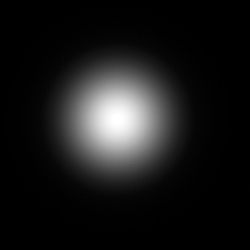
Figure 2-7 Environment Map of the Sun Overhead
The effect therefore calculates the normal of the wave function to trace the path of the ray to the intercept point on a plane—the ocean floor, in this example. To generate the normal, the partial derivatives of the wave function, in x and y, can easily be found.
Let's write the wave function used in the original approach as:
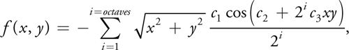
where i indicates the number of octaves used to generate the wave; c 1, c 2, and c 3 are constants to give the wave frequency, amplitude, and speed, respectively; and x and y, which range from 0 to 1, inclusive, indicate a point on a unit square.
Applying the chain and product rules yields two functions, the partial derivatives, which are written as: [1]
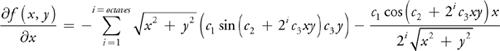
and
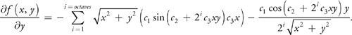
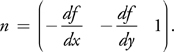
The partial derivatives are actually components of the gradient vectors at the point where they are evaluated. Because the function actually represents height, or z, the partial derivative with respect to z is simply 1. The normal is then the cross product of the gradient vectors, which yields:
The last equation required to render the caustics is the line-plane intercept. We can calculate the distance from a point on a line to the interception point on the plane using:
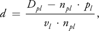
where Dpl is the distance from the water plane to the origin, npl is the normal of the ground plane, vl is the vector describing the direction of the refracted light (effectively along the normal of the wave surface), and pl is the intersection point of the refracted ray and the ocean floor. See Figure 2-8.
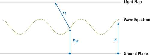
Figure 2-8 Accessing the Environment Map
Evidently the new calculations done per-pixel are quite complex, but given the flexibility of higher-level shading languages and the pixel-processing power available in current-generation hardware devices, they are trivial to implement and quick to render. The sample code in Listing 2-1 shows the implementation in Cg.
Example 2-1. Code Sample for the Wave Function, the Gradient of the Wave Function, and the Line-Plane Intercept Equation
// Caustics
// Copyright (c) NVIDIA Corporation. All rights reserved.
//
// NOTE:
// This shader is based on the original work by Daniel Sanchez-Crespo
// of the Universitat Pompeu Fabra, Barcelona, Spain.
#define VTXSIZE 0.01f
// Amplitude
#define WAVESIZE 10.0f
// Frequency
#define FACTOR 1.0f
#define SPEED 2.0f
#define OCTAVES 5
// Example of the same wave function used in the vertex engine
float wave(float x, float y, float timer)
{
  float z = 0.0f;
  float octaves = OCTAVES;
  float factor = FACTOR;
  float d = sqrt(x * x + y * y);
  do
  {
    z -= factor * cos(timer * SPEED + (1 / factor) * x * y * WAVESIZE);
    factor = factor / 2;
    octaves--;
  } while (octaves > 0);
  return 2 * VTXSIZE * d * z;
} // This is a derivative of the above wave function.
// It returns the d(wave)/dx and d(wave)/dy partial derivatives.
float2 gradwave(float x, float y, float timer)
{
  float dZx = 0.0f;
  float dZy = 0.0f;
  float octaves = OCTAVES;
  float factor = FACTOR;
  float d = sqrt(x * x + y * y);
  do
  {
    dZx +=
        d * sin(timer * SPEED + (1 / factor) * x * y * WAVESIZE) * y *
            WAVESIZE -
        factor * cos(timer * SPEED + (1 / factor) * x * y * WAVESIZE) * x / d;
    dZy +=
        d * sin(timer * SPEED + (1 / factor) * x * y * WAVESIZE) * x *
            WAVESIZE -
        factor * cos(timer * SPEED + (1 / factor) * x * y * WAVESIZE) * y / d;
    factor = factor / 2;
    octaves--;
  } while (octaves > 0);
  return float2(2 * VTXSIZE * dZx, 2 * VTXSIZE * dZy);
}
float3 line_plane_intercept(float3 lineP, float3 lineN, float3 planeN,
                            float planeD)
{
  // Unoptimized
  float distance = (planeD - dot(planeN, lineP)) / dot(lineN, planeN);
  // Optimized (assumes planeN always points up)
  float distance = (planeD - lineP.z) / lineN.z;
  return lineP + lineN * distance;
}
Once we have calculated the interception point, we can use this to fetch our caustic light map using a dependent texture read, and we can then add the caustic contribution to our ground texture, as shown in Listing 2-2.
Example 2-2. Code Sample for the Final Render Pass, Showing the Dependent Texture Read Operations
float4 main(VS_OUTPUT vert, uniform sampler2D LightMap
            : register(s0), uniform sampler2D GroundMap
            : register(s1), uniform float Timer)
    : COLOR
{
  // Generate a normal (line direction) from the gradient
  // of the wave function and intercept with the water plane.
  // We use screen-space z to attenuate the effect to avoid aliasing.
  float2 dxdy = gradwave(vert.Position.x, vert.Position.y, Timer);
  float3 intercept = line_plane_intercept(
      vert.Position.xyz, float3(dxdy, saturate(vert.Position.w)),
      float3(0, 0, 1), -0.8);
  // OUTPUT
  float4 colour;
  colour.rgb = (float3)tex2D(LightMap, intercept.xy * 0.8);
  colour.rgb += (float3)tex2D(GroundMap, vert.uv);
  colour.a = 1;
  return colour;
}
The results in Figure 2-9 show the quality improvement achieved by doing the calculations per-pixel instead of per-vertex. As can be seen, a sufficiently large resolution texture has quality as good as screen-space rendering, without the performance impact when large numbers of pixels are displayed. Additionally, when using a render target texture, we can take advantage of automatic mipmap generation and anisotropic filtering to reduce aliasing of the caustics, which cannot be done when rendering to screen space.
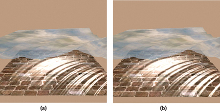
Figure 2-9 Rendered Caustics
2.6 Conclusion
The effect described in this chapter shows how a classic algorithm can be upgraded and enhanced to take advantage of shader-based techniques. As shader-processing power increases, the full Monte Carlo approach will eventually run entirely on graphics hardware, and thus computing physically correct caustics will become a reality.
For a complete, aesthetically pleasing model of underwater rendering, another effect worth investigating is crepuscular rays. This effect, also known as god rays, looks like visible rays of light, which are caused by reflections from underwater particles.
2.7 References
Foley, James, Andries van Dam, Steven Feiner, and John Hughes. 1996. Computer Graphics: Principles and Practice, 2nd ed. Addison-Wesley.
Jensen, Lasse Staff, and Robert Golias. 2001. "Deep-Water Animation and Rendering." Gamasutra article. Available online at http://www.gamasutra.com/gdce/2001/jensen/jensen_01.htm
Stam, Jos. 1996. "Random Caustics: Wave Theory and Natural Textures Revisited." Technical sketch. In Proceedings of SIGGRAPH 1996, p. 151. Available online at http://www.dgp.toronto.edu/people/stam/INRIA/caustics.html
Copyright
Many of the designations used by manufacturers and sellers to distinguish their products are claimed as trademarks. Where those designations appear in this book, and Addison-Wesley was aware of a trademark claim, the designations have been printed with initial capital letters or in all capitals.
The authors and publisher have taken care in the preparation of this book, but make no expressed or implied warranty of any kind and assume no responsibility for errors or omissions. No liability is assumed for incidental or consequential damages in connection with or arising out of the use of the information or programs contained herein.
The publisher offers discounts on this book when ordered in quantity for bulk purchases and special sales. For more information, please contact:
U.S. Corporate and Government Sales
(800) 382-3419
corpsales@pearsontechgroup.com
For sales outside of the U.S., please contact:
International Sales
international@pearsoned.com
Visit Addison-Wesley on the Web: www.awprofessional.com
Library of Congress Control Number: 2004100582
GeForce™ and NVIDIA Quadro® are trademarks or registered trademarks of NVIDIA Corporation.
RenderMan® is a registered trademark of Pixar Animation Studios.
"Shadow Map Antialiasing" © 2003 NVIDIA Corporation and Pixar Animation Studios.
"Cinematic Lighting" © 2003 Pixar Animation Studios.
Dawn images © 2002 NVIDIA Corporation. Vulcan images © 2003 NVIDIA Corporation.
Copyright © 2004 by NVIDIA Corporation.
All rights reserved. No part of this publication may be reproduced, stored in a retrieval system, or transmitted, in any form, or by any means, electronic, mechanical, photocopying, recording, or otherwise, without the prior consent of the publisher. Printed in the United States of America. Published simultaneously in Canada.
For information on obtaining permission for use of material from this work, please submit a written request to:
Pearson Education, Inc.
Rights and Contracts Department
One Lake Street
Upper Saddle River, NJ 07458
Text printed on recycled and acid-free paper.
5 6 7 8 9 10 QWT 09 08 07
5th Printing September 2007
- Contributors
- Copyright
- Foreword
- Part I: Natural Effects
-
- Chapter 1. Effective Water Simulation from Physical Models
- Chapter 2. Rendering Water Caustics
- Chapter 3. Skin in the "Dawn" Demo
- Chapter 4. Animation in the "Dawn" Demo
- Chapter 5. Implementing Improved Perlin Noise
- Chapter 6. Fire in the "Vulcan" Demo
- Chapter 7. Rendering Countless Blades of Waving Grass
- Chapter 8. Simulating Diffraction
- Part II: Lighting and Shadows
-
- Chapter 9. Efficient Shadow Volume Rendering
- Chapter 10. Cinematic Lighting
- Chapter 11. Shadow Map Antialiasing
- Chapter 12. Omnidirectional Shadow Mapping
- Chapter 13. Generating Soft Shadows Using Occlusion Interval Maps
- Chapter 14. Perspective Shadow Maps: Care and Feeding
- Chapter 15. Managing Visibility for Per-Pixel Lighting
- Part III: Materials
- Part IV: Image Processing
- Part V: Performance and Practicalities
-
- Chapter 28. Graphics Pipeline Performance
- Chapter 29. Efficient Occlusion Culling
- Chapter 30. The Design of FX Composer
- Chapter 31. Using FX Composer
- Chapter 32. An Introduction to Shader Interfaces
- Chapter 33. Converting Production RenderMan Shaders to Real-Time
- Chapter 34. Integrating Hardware Shading into Cinema 4D
- Chapter 35. Leveraging High-Quality Software Rendering Effects in Real-Time Applications
- Chapter 36. Integrating Shaders into Applications
- Part VI: Beyond Triangles
- Preface