GPU Gems
GPU Gems is now available, right here, online. You can purchase a beautifully printed version of this book, and others in the series, at a 30% discount courtesy of InformIT and Addison-Wesley.
The CD content, including demos and content, is available on the web and for download.
Chapter 5. Implementing Improved Perlin Noise
Ken Perlin
New York University
This chapter focuses on the decisions that I made in designing a new, improved version of my Noise function. I did this redesign for three reasons: (1) to make Noise more amenable to a gradual shift into hardware, (2) to improve on the Noise function's visual properties in some significant ways, and (3) to introduce a single, standard version that would return the same values across all hardware and software platforms.
The chapter is structured as follows: First, I describe the goals of the Noise function itself and briefly review the original implementation. Then I talk about specific choices I made in implementing improved Noise, to increase its quality and decrease visual artifacts. Finally, I talk about what is needed for gradual migration to hardware. The goal is to allow Noise to be implemented in progressively fewer instructions, as successive generations of GPUs follow a path to more powerful instructions.
5.1 The Noise Function
The purpose of the Noise function is to provide an efficiently implemented and repeatable, pseudo-random signal over R3 (three-dimensional space) that is band-limited (most of its energy is concentrated near one spatial frequency) and visually isotropic (statistically rotation-invariant).
The general idea is to create something that gives the same effect as a completely random signal (that is, white noise) that has been run through a low-pass filter to blur out and thereby remove all high spatial frequencies. One example is the gradually rising and falling hills and valleys of sand dunes, as shown in Figure 5-1.
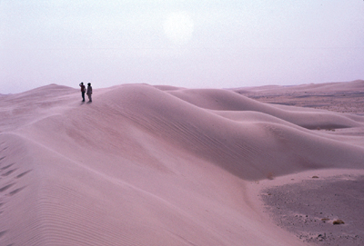
Figure 5-1 Sand Dunes
5.2 The Original Implementation
The initial implementation, first used in 1983 and first published in 1985 (Perlin 1985), defined Noise at any point (x, y, z) by using the following algorithm:
- At each point in space (i, j, k) that has integer coordinates, assign a value of zero and a pseudo-random gradient that is hashed from (i, j, k).
- Define the coordinates of (x, y, z) as an integer value plus a fractional remainder: (x, y, z) = (i + u, j + v, k + w). Consider the eight corners of the unit cube surrounding this point: (i, j, k), (i + 1, j, k), . . . (i + 1, j + 1, k + 1).
- Fit a Hermite spline through these eight points, and evaluate this spline at (x, y,
z), using u, v, and w as interpolants. If we use a table lookup to
predefine the Hermite cubic blending function 3t 2 - 2t 2,
then this interpolation requires only seven scalar linear interpolations: for example, four in x,
followed by two in y, followed by one in z, as shown in Figure 5-2.
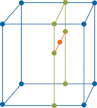
Figure 5-2 Steps Required to Interpolate a Value from Eight Samples in a Regular 3D Lattice
This approach worked reasonably well. A two-dimensional slice through the Noise function looks like Figure 5-3.
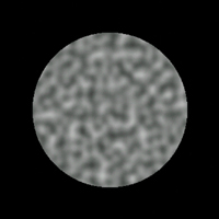
Figure 5-3 A Slice Through the Noise Function
5.3 Deficiencies of the Original Implementation
Unfortunately, Noise had the following deficiencies:
- The choice of interpolating function in each dimension was 3t 2 - 2t 3, which contains nonzero values in its second derivative. This can cause visual artifacts when the derivative of noise is taken, such as when doing bump mapping.
- The hashing of gradients from (i, j, k) produced a lookup into a pseudo-random
set of 256 gradient vectors sown on a 3D sphere; irregularities in this distribution produce unwanted higher
frequencies in the resulting Noise function. See Figure 5-4.
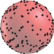
Figure 5-4 Irregular Distribution of Gradient Vectors
In retrospect, I realize I should have applied a relaxation algorithm in the preprocessing step that chooses the pseudo-random gradient directions, repulsing these points away from each other around the sphere to form a more even, Poisson-like distribution, which would have reduced unwanted high spatial frequencies, giving a result like the one visualized in Figure 5-5.
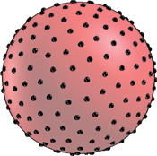
Figure 5-5 Regular Distribution of Gradient Vectors
Recently I realized that such a large number of different gradient directions is not even visually necessary. Rather, it is far more important to have an even statistical distribution of gradient directions, as opposed to many different gradient directions. This is consistent with perceptual research demonstrating that although human pre-attentive vision is highly sensitive to statistical anomalies in the orientation of texture features, our vision is relatively insensitive to the granularity of orientations, because our low-level vision system will convert a sufficiently dense set of discrete orientations into the equivalent continuous signal (Grill Spector et al. 1995). The human vision system performs this conversion at a very early stage, well below the threshold of conscious awareness.
Given a Noise implementation with a statistically even distribution of gradient directions, it is fairly straightforward to build procedural expressions that create complex-looking textures. For example, Figure 5-6 shows four successively more complex texture expressions built from Noise.
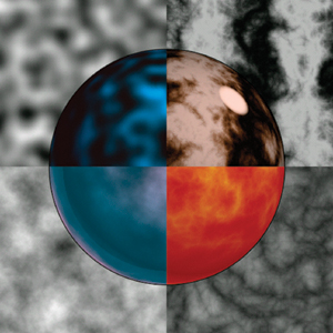
Figure 5-6 Four Texture Expressions Built from Noise
Moving clockwise from the top left, these expressions are:
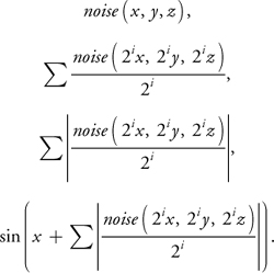
In each case, color splines have been applied as a postprocess to tint the results.
5.4 Improvements to Noise
The improvements to the Noise function are in two specific areas: the nature of the interpolant and the nature of the field of pseudo-random gradients.
As I discussed in Perlin 2002, the key to improving the interpolant is simply to remove second-order discontinuities. The original cubic interpolant 3t 2 - 2t 3 was chosen because it has a derivative of zero both at t = 0 and at t = 1. Unfortunately, its second derivative is 6 - 12t, which is not zero at either t = 0 or at t = 1. This causes artifacts to show up when Noise is used in bump mapping. Because the effect of lighting upon a bump-mapped surface varies with the derivative of the corresponding height function, second-derivative discontinuities are visible.
This problem was solved by switching to the fifth-degree interpolator: 6t 5 - 15t 4 + 10t 3, which has both first and second derivatives of zero at both t = 0 and t = 1.
The difference between these two interpolants can be seen in Figure 5-7. The green curve is the old cubic interpolant, which has second-order discontinuities at t = 0 and t = 1. The blue curve is the new fifth-order interpolant, which does not suffer from second-order discontinuities at t = 0 and t = 1.
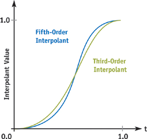
Figure 5-7 Interpolation Curves
One nice thing about graphics accelerators is that you perform one-dimensional interpolations via a one-dimensional texture lookup table. When you take this approach, there is no extra cost in doing the higher-order interpolation. In practice, I have found that a texture table length of 256 is plenty, and that 16 bits of precision is sufficient. Even half-precision floating point (fp16), with its 10-bit mantissa, is sufficient.
Figure 5-8 shows two different renderings of a Noise-displaced superquadric. The one on the left uses the old cubic interpolant; the one on the right uses the newer, fifth-order interpolant. The visual improvement can be seen as a reduction in the 4x4-grid-like artifacts in the shape's front face.
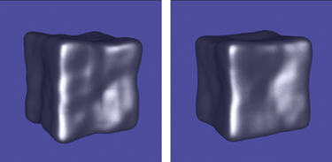
Figure 5-8 Noise-Displaced Superquadric
The other improvement was to replace the 256 pseudo-random gradients with just 12 pseudo-random gradients, consisting of the edge centers of a cube centered at the origin: (0, ±1, ±1), (±1, 0, ±1), and (±1, ±1, 0). This results in a much less "splotchy-looking" distribution, as can be seen in Figure 5-9's side-by-side comparison of a planar slice taken from implementations of Noise using the old and the new approach.
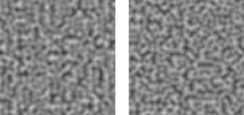
Figure 5-9 Improving Gradient Distribution
The reason for this improvement is that none of the 12 gradient directions is too near any others, so they will never bunch up too closely. It is this unwanted bunching up of adjacent gradients that causes the splotchy appearance in parts of the original Noise implementation.
Another nice thing about this approach is that it makes it possible to avoid many of the multiplies associated with evaluating the gradient function, because an inner product of (x, y, z) with, say, (1, 1, 0) can be computed simply as x + y.
In order to make the process of hashing into this set of gradients compatible with the fastest possible hardware implementation, 16 gradients are actually defined, so that the hashing function can simply return a random 4-bit value. The extra four gradients simply repeat (1, 1, 0), (-1, 1, 0), (0, -1, 1), and (0, -1, -1).
5.5 How to Make Good Fake Noise in Pixel Shaders
It would be great to have some sort of reasonable volumetric noise primitive entirely in a pixel shader, but the straightforward implementation of this takes quite a few instructions. How can we use the capabilities of today's pixel shaders to implement some reasonable approximation of Noise in a very small number of instructions? Suppose we agree that we're willing to use piecewise trilinear rather than higher polynomial interpolation (because today's GPUs provide direct hardware acceleration of trilinear interpolation), and that we're willing to live with the small gradient discontinuities that result when you use trilinear interpolation.
One solution would be to place an entire volume of noise into a trilinear-interpolated texture. Unfortunately, this would be very space intensive. For example, a cube sampling noise from (0, 0, 0) through (72, 72, 72), containing three samples per linear unit distance plus one extra for the final endpoint, or (3 x 72) + 1 samples in each direction, would require 217 x 217 x 217 = 10,218,313 indexed locations, which is inconveniently large.
But the fact that today's GPUs can perform fast trilinear interpolation on reasonably small-size volumes can be exploited in a different way. For example, an 8x8x8 volume sampled the same way requires (3 x 8) + 1 samples in each direction, or only 25x25x25 = 15,625 indexed locations. What I've been doing is to define noise through multiple references into such modest-size stored volumes.
So how do you get a 723 cube out of an 83 cube? The trick is to do it in two steps:
- Fill the space with copies of an 83 sample that is a toroidal tiling. In other words, construct this sample so that it forms an endlessly repeating continuous pattern, with the top adjoining seamlessly to the bottom, the left to the right, and the back to the front. When these samples are stacked in space as cubic bricks, they will produce a continuous but repeating, space-filling texture.
- Use this same sampled pattern, scaled up by a factor of nine, as a low-frequency pattern that varies this fine-scale brick tiling in such a way that the fine-scale pattern no longer appears to be repeating.
The details are as follows: Rather than define the values in this repeating tile as real numbers, define them as complex values. Note that this doubles the storage cost of the table (in this case, to 31,250 indexed locations). If we use a 16-bit quantity for each numeric scalar in the table, then the total required memory cost is 31,250x2x2 bytes = 125,000 bytes to store the volume.
Evaluate both the low-frequency and the high-frequency noise texture. Then use the real component of the low-frequency texture as a rotational phase shift as follows: Let's say we have retrieved a complex value of (lor , loi ) from the low-frequency texture and a complex value of (hir , hii ) from the high-frequency texture. We use the low-frequency texture to rotate the complex value of the high-frequency texture by evaluating the expression:

The three images in Figure 5-10 show, in succession, (a) the real component of a planar slice through the high-frequency texture, (b) the real component of a planar slice through the low-frequency texture, and (c) the final noise texture obtained by combining them.
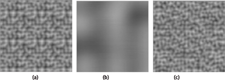
Figure 5-10 Combining High-Frequency and Low-Frequency Textures
Notice that the visible tiling pattern on the leftmost image is no longer visible in the rightmost image.
5.6 Making Bumps Without Looking at Neighboring Vertices
Once you can implement Noise directly in the pixel shader, then you can implement bump mapping as follows:
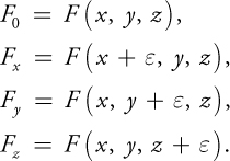
- Consider a point (x, y, z) and some function F(x, y, z) that you've defined in your pixel shader through some combination of noise functions.
- Choose some small value of e and compute the following quantities:
- This allows a good approximation of the gradient (or derivative) vector of F at (x,
y, z) by:
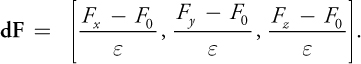
- Subtract this gradient from your surface normal and then renormalize the result back to unit length:
N = normalize(N - dF)
Figure 5-11 shows the result of applying exactly this approach to three different procedural bump maps on a sphere: a simple lumpy pattern, an embossed marble pattern, and a fractal crinkled pattern.
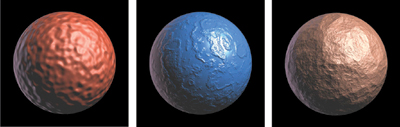
Figure 5-11 Bump Mapping a Sphere
Assuming that the model is a unit-radius sphere, the expressions that implement these bump patterns:
.03 * noise(x, y, z, 8); // LUMPY
.01 * stripes(x + 2 * turbulence(x, y, z, 1), 1.6);
// MARBLE
- .10 * turbulence(x, y, z, 1);
// CRINKLED
are defined atop the following functions:
// STRIPES TEXTURE (GOOD FOR MAKING MARBLE)
double stripes(double x, double f)
{
  double t = .5 + .5 * sin(f * 2 * PI * x);
  return t * t - .5;
}
// TURBULENCE TEXTURE
double turbulence(double x, double y, double z, double f)
{
  double t = -.5;
  for (; f < = W / 12; f *= 2) // W = Image width in pixels
    t += abs(noise(x, y, z, f) / f);
  return t;
}
5.7 Conclusion
Procedural texturing using volumetric noise is extremely useful in situations where you want to create an impression of natural-looking materials, without the necessity of creating an explicit texture image. Also, rather than trying to figure out how to map a texture image parametrically onto the surface of your shape, the volumetric nature of noise-based textures allows you simply to evaluate them at the (x, y, z) locations in your pixel shader. In this way, you are effectively carving your texture out of a solid material, which is often much more straightforward than trying to work out a reasonable undistorted parametric mapping.
Noise-based textures also allow you to work in a resolution-independent way: rather than the texture blurring out when you get nearer to an object, it can be kept crisp and detailed, as you add higher frequencies of noise to your texture-defining procedure.
As is always the case with procedural textures, you should try not to add very high frequencies that exceed the pixel sample rate. Such super-pixel frequencies do not add to the visual quality, and they result in unwanted speckling as the texture animates.
The key to being able to use noise-based textures efficiently on GPUs is the availability of an implementation of noise that really makes use of the enormous computational power of GPUs. Here we have outlined such an implementation, and shown several examples of how it can be used in your pixel shader to procedurally define bump maps.
These sorts of volumetric noise-based procedural textures have long been mainstays of feature films, where shaders do not require real-time performance, yet do require high fidelity to the visual appearance of natural materials. In fact, all special-effects films today make heavy use of noise-based procedural shaders. The convincing nature of such effects as the ocean waves in A Perfect Storm and the many surface textures and atmosphere effects in The Lord of the Rings trilogy, to take just two examples, is highly dependent on the extensive use of the noise function within pixel shaders written in languages such as Pixar's RenderMan. With a good implementation of the noise function available for real-time use in GPUs, I look forward to seeing some of the exciting visual ideas from feature films incorporated into the next generation of interactive entertainment on the desktop and the console.
5.8 References
Grill Spector, K., S. Edelman, and R. Malach. 1995. "Anatomical Origin and Computational Role of Diversity in the Response Properties of Cortical Neurons." In Advances in Neural Information Processing Systems 7, edited by G. Tesauro, D. S. Touretzky, and T. K. Leen. MIT Press.
Perlin, K. 1985. "An Image Synthesizer." Computer Graphics 19(3).
Perlin, K. 2002. "Improving Noise." Computer Graphics 35(3).
Copyright
Many of the designations used by manufacturers and sellers to distinguish their products are claimed as trademarks. Where those designations appear in this book, and Addison-Wesley was aware of a trademark claim, the designations have been printed with initial capital letters or in all capitals.
The authors and publisher have taken care in the preparation of this book, but make no expressed or implied warranty of any kind and assume no responsibility for errors or omissions. No liability is assumed for incidental or consequential damages in connection with or arising out of the use of the information or programs contained herein.
The publisher offers discounts on this book when ordered in quantity for bulk purchases and special sales. For more information, please contact:
U.S. Corporate and Government Sales
(800) 382-3419
corpsales@pearsontechgroup.com
For sales outside of the U.S., please contact:
International Sales
international@pearsoned.com
Visit Addison-Wesley on the Web: www.awprofessional.com
Library of Congress Control Number: 2004100582
GeForce™ and NVIDIA Quadro® are trademarks or registered trademarks of NVIDIA Corporation.
RenderMan® is a registered trademark of Pixar Animation Studios.
"Shadow Map Antialiasing" © 2003 NVIDIA Corporation and Pixar Animation Studios.
"Cinematic Lighting" © 2003 Pixar Animation Studios.
Dawn images © 2002 NVIDIA Corporation. Vulcan images © 2003 NVIDIA Corporation.
Copyright © 2004 by NVIDIA Corporation.
All rights reserved. No part of this publication may be reproduced, stored in a retrieval system, or transmitted, in any form, or by any means, electronic, mechanical, photocopying, recording, or otherwise, without the prior consent of the publisher. Printed in the United States of America. Published simultaneously in Canada.
For information on obtaining permission for use of material from this work, please submit a written request to:
Pearson Education, Inc.
Rights and Contracts Department
One Lake Street
Upper Saddle River, NJ 07458
Text printed on recycled and acid-free paper.
5 6 7 8 9 10 QWT 09 08 07
5th Printing September 2007
- Contributors
- Copyright
- Foreword
- Part I: Natural Effects
-
- Chapter 1. Effective Water Simulation from Physical Models
- Chapter 2. Rendering Water Caustics
- Chapter 3. Skin in the "Dawn" Demo
- Chapter 4. Animation in the "Dawn" Demo
- Chapter 5. Implementing Improved Perlin Noise
- Chapter 6. Fire in the "Vulcan" Demo
- Chapter 7. Rendering Countless Blades of Waving Grass
- Chapter 8. Simulating Diffraction
- Part II: Lighting and Shadows
-
- Chapter 9. Efficient Shadow Volume Rendering
- Chapter 10. Cinematic Lighting
- Chapter 11. Shadow Map Antialiasing
- Chapter 12. Omnidirectional Shadow Mapping
- Chapter 13. Generating Soft Shadows Using Occlusion Interval Maps
- Chapter 14. Perspective Shadow Maps: Care and Feeding
- Chapter 15. Managing Visibility for Per-Pixel Lighting
- Part III: Materials
- Part IV: Image Processing
- Part V: Performance and Practicalities
-
- Chapter 28. Graphics Pipeline Performance
- Chapter 29. Efficient Occlusion Culling
- Chapter 30. The Design of FX Composer
- Chapter 31. Using FX Composer
- Chapter 32. An Introduction to Shader Interfaces
- Chapter 33. Converting Production RenderMan Shaders to Real-Time
- Chapter 34. Integrating Hardware Shading into Cinema 4D
- Chapter 35. Leveraging High-Quality Software Rendering Effects in Real-Time Applications
- Chapter 36. Integrating Shaders into Applications
- Part VI: Beyond Triangles
- Preface