GPU Gems

GPU Gems is now available, right here, online. You can purchase a beautifully printed version of this book, and others in the series, at a 30% discount courtesy of InformIT and Addison-Wesley.

The CD content, including demos and content, is available on the web and for download.

Chapter 20. Texture Bombing

R. Steven Glanville
NVIDIA

Textures are useful for adding visual detail to geometry, but they don't work as well when extended to cover large areas such as a field of flowers, or many similar objects such as a city full of buildings. Such uses require either a very large amount of texture data or repetition of the same pattern, resulting in an undesirable, regular look. Texture bombing is a procedural technique that places small images at irregular intervals to help reduce such pattern artifacts.

20.1 Texture Bombing 101

The basic idea behind texture bombing is to divide UV space into a regular grid of cells. We then place an image within each cell at a random location, using a noise or pseudo-random number function. The final result is the composite of these images over the background.

It's not very efficient to actually composite images in this manner, because we may have hundreds of images to combine. We may also want to compute the image procedurally, which is somewhat incompatible with compositing. We'll discuss both techniques in this chapter. To start, let's view things from a pixel's perspective and try to pare down the work. The first step is to find the cell containing the pixel. We need to compute each cell's coordinates in a way that lets us quickly locate neighbor cells, as you will see later on. We'll use these coordinates to access all of the cell's unique parameters, such as the image's location within that cell. Finally, we sample the image at its location within the cell and combine it with a default background color. We assume here that a sample is either 100 percent opaque or transparent, to simplify the compositing step.

It's not quite this simple, however. If a cell's image is located close to the edge of its cell, or if it is larger than a cell, it will cross into adjacent cells. Therefore, we need to consider neighboring cells' images as well. Large cell images would require that we sample many adjacent images. If we limit the image size to be no bigger than a cell, then we need to sample only nine cells: both side cells, those above and below, and the four cells at the corners. We can reduce the number of required samples to four by introducing a few minor restrictions on the images.

20.1.1 Finding the Cell

The cell's coordinates are computed simply, using a floor function of the pixel's UV parameters:

 float2 scaledUV = UV * scale; int2 cell = floor(scaledUV);

Note that the cell's coordinates are integral. Adjacent cells differ by 1 in either cell.x or cell.y. The scale factor allows us to vary the size as needed. Finding our location within the cell simply requires a subtraction:

 float2 offset = scaledUV - cell;

20.1.2 Sampling the Image

Before we can sample the image, we need to determine its location. We use a two-dimensional texture filled with pseudo-random numbers for this task. The coordinates for the sample are derived from the cell's coordinates, scaled by small values.

 float2 randomUV = cell * float2(0.037, 0.119); fixed4 random = tex2D(randomTex, randomUV);

There's nothing magic about the scale factors used to compute randomUV. They map the integral cell name to somewhere within the random texture and should have the property of mapping nearby cells to uncorrelated values. Any value large enough to separate adjacent cells a distance of more than one texel should suffice.

We use the first two components of the texture for the image's location within the cell, which must be subtracted from the pixel's offset within the cell. If the alpha component of the image is not zero, then the image's color is used; otherwise, the original color is used.

 fixed4 image = tex2D(imageTex, offset.xy - random.xy); if (image.w > 0.0)   color.xyz = image.xyz;

Putting this together into sample program texbomb_1.cg, and using the background and image patterns in Figure 20-1a and 20-1b, yields the result shown in Figure 20-1c. (All the sample programs shown in this chapter are included on the book's CD and are available on the book's Web site.)

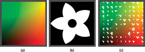
Figure 20-1 First Attempt at Texture Bombing

It's not quite there. The images are clipped by the edges of the cell. The only time that the full image is visible is when its offset is zero. We also have to look for images in adjacent cells.

20.1.3 Adjacent Cells' Images

So far we've sampled only the current cell's image. We also need to check for overlapping images from adjacent cells. Because we've limited the image offset relative to a cell to be in the range 0 to 1, an image can overlap only those cells above and to the right of its home cell. Thus we need sample only four cells: the current cell plus those cells below and to the left of our cell. See Listing 20-1.

Example 20-1. Extending the Sampling to Four Cells

 for (i = -1; i <= 0; i++) {   for (j = -1; j <= 0; j++) {     float2 cell_t = cell + float2(i, j);     float2 offset_t = offset - float2(i, j);     randomUV = cell_t.xy * float2(0.037, 0.119);     random = tex2D(randomTex, randomUV);     image = tex2D(imageTex, offset_t - random.xy);     if (image.w > 0.0)       color = image;     }   } }

20.1.4 Image Priority

There's something not quite right. When two images overlap, the one to the upper right is always on top, because it was the last one tested. This might be acceptable for scales on a fish or shingles, but we'd generally like to avoid this effect. Introducing a priority for each cell, in which the highest priority image wins, solves this problem. We use the w component of the cell's random parameter for the priority and change the if test from Listing 20-1 to that shown in Listing 20-2.

Example 20-2. Adding Image Priority

 fixed priority = -1; . . . if (random.w > priority && image.w > 0.0) {   color = image;   priority = random.w; }

Figure 20-2 shows an image from this revised program, called texbomb_2.cg.

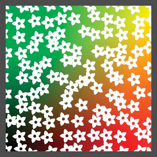
Figure 20-2 The Output of

20.1.5 Procedural Images

There is no reason that the image has to come from a texture. Procedural images work just as well. In Listing 20-3, we've replaced the image sample with a procedurally generated circle of radius 0.5.

Example 20-3. Using a Procedurally Generated Circle

 offset_t -= float2(0.5, 0.5) + (float2) random; fixed radius2 = dot(offset_t, offset_t); if (random.w > priority && radius2 < 0.25) {   color = tex2D(randomTex, randomUV + float2(0.13, 0.4));   priority = random.w; }

A second sample of the random texture gives the circle's color, as shown in Figure 20-3, produced from the program gem_proc_2.cg.

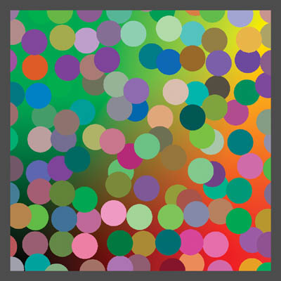
Figure 20-3 The Output of

Multiple Images per Cell

Using only one image per cell can lead to a regular-looking pattern, especially when the cells are small. There isn't enough variance to hide the grid nature of the computation, making the distribution look too regular. To counter this tendency, we can increase the number of images in each cell by simply adding a loop around the image sample and offsetting the coordinates used for looking up the random numbers. See Listing 20-4.

Example 20-4. Sampling Multiple Circles per Cell Reduces Grid-Like Patterns

 randomUV = cell_t.xy * float2(0.037, 0.119); for (k = 0; k < NUMBER_OF_SAMPLES; k++) {   random = tex2D(randomTex, randomUV);   randomUV += float2(0.03, 0.17);   image = tex2D(imageTex, offset_t - random.xy);   . . . }

We offset the coordinates for each pass in the loop to prevent sampling the same value each time. See Figure 20-4.

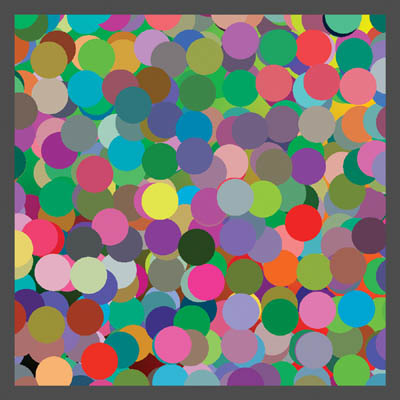
Figure 20-4 Sampling Three Circles per Cell

We can also vary the number of images per cell by using another random value, or even by simply setting the initial priority to something higher than 0, such as 0.5. Then each image has a probability of 0.5 that it will be rejected. This variation further increases the apparent randomness of the result, as shown in Figure 20-5. Here the size of the cells has been reduced to show a larger number.

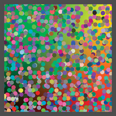
Figure 20-5 Varying the Number of Circles per Cell

20.1.6 Random Image Selection from Multiple Choices

Another dimension of variation can be added by selecting from one of multiple images for each choice. One way to do this is to tile the images into a single texture and use the z component of the random texture as an index into these images. It's simpler to arrange the images in a single horizontal row, as shown in Figure 20-6. The black area corresponds to the transparent region and has an alpha component of zero.

Figure 20-6 Storing Four Images in a Single Texture Map

Then all we need to do is change the image lookup call to select from one of four sub-images. Scaling the z component of the random vector and computing the floor yields an integer index of a random image. We need to clamp the x coordinate to prevent adjacent images from being sampled, add the value of index, and scale by 1/number of images.

 float index = floor(random.z * NUM_IMAGES_PER_ROW); float2 uv = offset_t.xy - random.xy; uv.x = (saturate(uv.x) + index) / NUM_IMAGES_PER_ROW; image = tex2D(imageTex, uv);

The result is shown in Figure 20-7. Note that the images need at least a two-pixel border separating them from the edges of their region, or else texture sampling will cause artifacts.

Figure 20-7 Random Image Selection

If ordinary mipmaps are used for a multiple-image texture, then a two-pixel border between images won't be sufficient. A sample near an image's edge taken from a higher-level map can blend with the adjacent image. You can reduce such problems by increasing the width of the border, or by constructing the mipmaps with a similar border at each level. You may also want to clamp the maximum mipmap level to avoid degenerate cases, or you can simply reduce the image size to zero.

20.2 Technical Considerations

There are a couple of implementation details that need discussing.

It is important to choose the right minification filter used for the random-number texture. When mipmapping is enabled, dependent texture reads such as those used to get the pseudo-random numbers generate a level of detail (LOD) based on the difference of the UV values in the current and adjacent pixels. Within a cell, randomUV is the same for all pixels. The difference is therefore zero and LOD 0 is sampled, yielding a (possibly bilinearly interpolated) value from the original random numbers. However, at the boundary between two cells, the value of randomUV changes abruptly. Thus, a higher mipmap level is used, and an artifact is introduced.

Specifying a minification filter of LINEAR or NEAREST for the random texture eliminates these artifacts, because they force all samples to LOD 0. It's better to use a NEAREST filter for static textures. A LINEAR filter reduces the variance of the random numbers and tends to keep the images closer to the center of their cells. But if you are animating the images' positions, then you will want to use LINEAR for smooth motion.

The wrap mode for the texture image should be set to CLAMP. Otherwise, we'll see ghost samples where we shouldn't. Alternatively, we can clamp the coordinates to the range [0..1]. Most GPUs have hardware to do this at no cost.

20.2.1 Efficiency Issues

Reducing execution time is always important for pixel shaders, and texture bombing is no exception. Dependent texture samples, repeated evaluation of the basic shading for multiple cells, and even multiple samples per cell combine to hinder performance. The resulting shaders can be hundreds of instructions in length.

For example, the complete daisy image from texbomb_2.cg shown earlier in Figure 20-2 requires eight texture samples and 44 math instructions. The first procedural image from gem_proc_2.cg, shown earlier in Figure 20-3, requires eight texture samples and 62 math instructions.

Some key optimizations can help performance considerably. When possible, move the final color texture sample out of the inner loop. Instead of sampling the texture multiple times, save the coordinates of the resulting sample in a variable and do one final sample at the end of the program. This works well for procedural shapes, such as circles, and for Voronoi-like regions, because the decision to use a particular color is not based on the value of that sample. (See Section 20.3.5 for more on Voronoi regions.) Unfortunately, this trick does not work for an image when you need the alpha component to determine if that value is transparent or not.

On GeForce FX hardware, use fixed and half-precision variables when possible. This allows more instructions to be executed per shader pass and reduces the number of registers needed to run a program. Unless you are rendering to a float frame buffer, colors fit well in less precision. Texture coordinates, however, normally should be stored in full float precision.

20.3 Advanced Features

Texture bombing can be extended in a variety of ways for an interesting range of effects.

20.3.1 Scaling and Rotating

One simple addition is to randomly scale or rotate each image for further variation. You must be careful to stay within the area sampled by the adjacent cells that the image can cover. For scaling, it's fairly obvious that you can only reduce the size, unless you are willing to test more than four cells per pixel.

Rotated images have similar limitations. The opaque part of the image should lie within a circle of diameter 1 centered in the cell. If it were to exceed this size into the corners, then these portions of the rotated image could extend farther than 0.5 cells width vertically or horizontally from their base cell. The four-cell sample algorithm would miss these parts as well.

20.3.2 Controlled Variable Density

Sometimes you want to control artistically the pattern of, say, leaves on the ground. Using a pseudo-random density doesn't handle this case well. Instead, you can use a specific density texture and paint the probability for a leaf to appear as you wish. This texture would be read as a normal UV-based sample, and that value would be used, as in the preceding example, to set the probability that a leaf appears.

20.3.3 Procedural 3D Bombing

Once you've decided to use procedural textures, there's really no reason to limit the cells to a 2D UV space. Why not extend the idea into 3D using the object-space coordinates of a pixel to derive the color? In Listing 20-5, we divide object space into unit cubes. We can still use a 2D pseudo-random texture, but we need to include the third dimension as a component in computing the sample's coordinates. Scaling the z coordinate and adding it to the x and y gives a good result.

Example 20-5. Procedural 3D Bombing

 for (i = -1; i <= 0; i++) {   for (j = -1; j <= 0; j++) {     for (k = -1; k <= 0; k++) {       cell_t = cell + float3(i, j, k);       offset_t = offset - float3(i, j, k);       randomUV = cell_t.xy * float2(0.037, 0.119) +                    cell_t.z * 0.003;       . . .     }   } }

You have to extend the number of cells sampled to three dimensions as well, for a total of eight samples. Three-dimensional texture bombing is inherently more expensive than 2D for this reason. The example in Figure 20-8 shows procedurally generated spheres. It uses a simple dot-product diffuse-lighting model to show the depth.

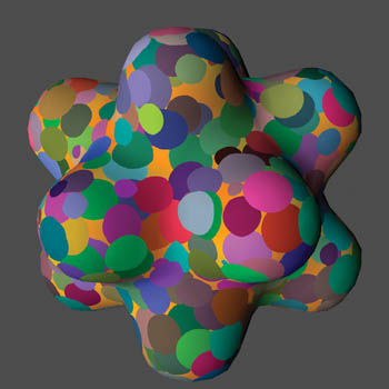
Figure 20-8 A Procedural 3D Texture with One Sphere per Cell

The full shader body is shown in Listing 20-6, for clarity.

Example 20-6. The Procedural 3D Texture Program

 priority = -1; for (i = -1; i <= 0; i++) {   for (j = -1; j <= 0; j++) {     for (k = -1; k <= 0; k++) {       cell_t = cell + float3(i, j, k);       offset_t = offset - float3(i, j, k);       randomUV = cell_t.xy * float2(0.037, 0.119) +                    cell_t.z * 0.003;       random = tex2D(randomTex, randomUV);       offset_t3 = offset_t -(float3(0.5, 0.5, 0.5) +                              (float3) random);       radius2 = dot(offset_t3, offset_t3);       if (random.w > priority && radius2 < 0.5) {         color = tex2D(randomTex, randomUV + float2(0.13, 0.4));         priority = random.w;       }     }   } } 
float factor = dot(normal.xyz, float3(0.5, 0.75, -0.3)) * 0.7 + 0.3; color.xyz = color.xyz * factor; return color;

20.3.4 Time-Varying Textures

You can easily animate texture-bombed shaders. All that's required is varying one or more of the pseudo-random parameters based on time. If you sample the pseudo-random number texture with a bilinear filter, then many properties will animate fairly smoothly. However, you may sometimes notice the ramp-like nature of this filtering, especially for moving objects, because the human eye is good at detecting discontinuities in the direction of motion.

 random = tex2D(randomTex, randomUV * time * 0.0001);

In the code shown here, the value of time is expressed in seconds. The animation would go by too quickly if it were not scaled down by an appropriate factor. The scale factor depends on the rate of the animation and the size of the pseudo-random texture. If the texture used in the example is 1024 by 1024, then a new texel will be sampled approximately every 10 seconds:

rate of change = (scale factor x time) / texture size.

20.3.5 Voronoi-Related Cellular Methods

An interesting variation on texture bombing is depicting Voronoi regions on a plane. See Steven Worley's 1996 SIGGRAPH paper for more information about this texturing technique. In a nutshell, given a plane and a set of points on that plane, a point's Voronoi region is the area in the plane that is closest to that particular point. You can see examples of Voronoi-like patterns in the shapes of cells on leaves or skin, cracks in dried mud, and to a certain extent in reptilian skin patterns, though these tend to be more regular. A typical view of Voronoi regions is shown in Figure 20-9.

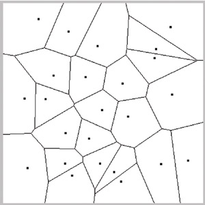
Figure 20-9 Sample Voronoi Regions

We can make these patterns with a small change to the basic texture-bombing code. Starting with the procedural circles' code shown earlier in Listing 20-3, we'll use the distance to a point as the priority, instead of the value in random.w, and we won't check to see if we're outside the radius of our circle. See Listing 20-7.

We use the square of the distance instead of the actual distance to avoid computing a square root. Each region is given a randomly assigned color. The result is shown in Figure 20-10a.

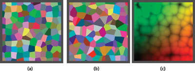
Figure 20-10 Voronoi Regions

Example 20-7. Computing Voronoi Regions

 float priority = 999; . . . radius2 = dot(offset_t2, offset_t2); if (radius2 < priority) {   color = tex2D(randomTex, randomUV + float2(0.13, 0.4));   priority = radius2; }

Notice that the rectangular grid structure of the algorithm is fairly apparent in Figure 20-10a. By increasing the number of samples, we can reduce this regularity considerably. Figure 20-10b uses three samples per cell, with cells scaled by a factor of sqrt(3) to keep the average Voronoi region size the same.

On a technical note, the cells created by this algorithm aren't guaranteed to be Voronoi regions. The point in a neighboring cell, P_n , can be in the opposite corner from our sample, but the point in the cell past that, P_n ₊₁, may be on the close edge, such that P_n ₊₁ is actually closer. However, we don't include the cell belonging to P_n ₊₁ in our computations. Practically speaking, this doesn't happen very often, and the regions are still useful. Increasing the number of samples per cell reduces the probability of this problem occurring.

You can create many interesting effects with these cells. Figure 20-10c has the same cell pattern as Figure 20-10b, but it uses the square of the distance from the closest point to modulate the background color.

20.4 Conclusion

Texture bombing and related cellular techniques can add visual richness to your shaders. Using a table of pseudo-random numbers stored in a texture, and a little programming, you can amplify the variability of an image or a set of images and reduce the repetitive look of large textured regions.

20.5 References

Apodaca, A. A., and L. Gritz. 2002. Advanced RenderMan, pp. 255–261. Morgan Kaufmann.

Ebert, D. S., F. K. Musgrave, D. Peachy, K. Perlin, and S. Worley. 2003. Texturing and Modeling: A Procedural Approach, 3rd ed., pp. 91–94. Morgan Kaufmann.

Lefebvre, S., and F. Neyret. 2003. "Pattern Based Procedural Textures." ACM Symposium on Interactive 3D Graphics 2003.

Schacter, B. J., and N. Ahuja. 1979. "Random Pattern Generation Processes." Computer Graphics and Image Processing 10, pp. 95–114.

Worley, Steven P. 1996. "A Cellular Texture Basis Function." In Proceedings of SIGGRAPH 96, pp. 291–294.

Copyright

Many of the designations used by manufacturers and sellers to distinguish their products are claimed as trademarks. Where those designations appear in this book, and Addison-Wesley was aware of a trademark claim, the designations have been printed with initial capital letters or in all capitals.

The authors and publisher have taken care in the preparation of this book, but make no expressed or implied warranty of any kind and assume no responsibility for errors or omissions. No liability is assumed for incidental or consequential damages in connection with or arising out of the use of the information or programs contained herein.

The publisher offers discounts on this book when ordered in quantity for bulk purchases and special sales. For more information, please contact:

U.S. Corporate and Government Sales
(800) 382-3419
corpsales@pearsontechgroup.com

For sales outside of the U.S., please contact:

International Sales
international@pearsoned.com

Visit Addison-Wesley on the Web: www.awprofessional.com

Library of Congress Control Number: 2004100582

GeForce™ and NVIDIA Quadro^® are trademarks or registered trademarks of NVIDIA Corporation.
RenderMan^® is a registered trademark of Pixar Animation Studios.
"Shadow Map Antialiasing" © 2003 NVIDIA Corporation and Pixar Animation Studios.
"Cinematic Lighting" © 2003 Pixar Animation Studios.
Dawn images © 2002 NVIDIA Corporation. Vulcan images © 2003 NVIDIA Corporation.

All rights reserved. No part of this publication may be reproduced, stored in a retrieval system, or transmitted, in any form, or by any means, electronic, mechanical, photocopying, recording, or otherwise, without the prior consent of the publisher. Printed in the United States of America. Published simultaneously in Canada.

For information on obtaining permission for use of material from this work, please submit a written request to:

Pearson Education, Inc.
Rights and Contracts Department
One Lake Street
Upper Saddle River, NJ 07458

Text printed on recycled and acid-free paper.

5 6 7 8 9 10 QWT 09 08 07

5th Printing September 2007

Part II: Lighting and Shadows

Part III: Materials

Part IV: Image Processing

Part V: Performance and Practicalities

Part VI: Beyond Triangles

Preface