GPU Gems

GPU Gems is now available, right here, online. You can purchase a beautifully printed version of this book, and others in the series, at a 30% discount courtesy of InformIT and Addison-Wesley.

The CD content, including demos and content, is available on the web and for download.

Chapter 13. Generating Soft Shadows Using Occlusion Interval Maps

William Donnelly
University of Waterloo

Joe Demers
NVIDIA

In this chapter we present a technique for rendering soft shadows that we call occlusion interval mapping. Occlusion interval maps were used to produce soft shadows in the NVIDIA GeForce FX 5900 demo "Last Chance Gas." See Figure 13-1. We call the technique occlusion interval mapping because it uses texture maps to store intervals that represent when the light source is visible and when it is occluded. In situations that satisfy the algorithm's requirements, occlusion interval mapping allows you to achieve impressive visual results at high frame rates.

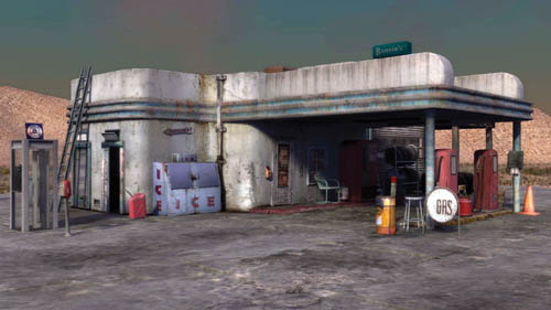
Figure 13-1 The "Last Chance Gas" Demo

13.1 The Gas Station

One of the goals of the GeForce FX 5900 demo "Last Chance Gas" was to create a scene with accurate outdoor lighting. One important aspect of outdoor lighting we wanted to capture is soft shadows from the Sun. Unlike the hard shadows produced by shadow maps or stencil shadow volumes, soft shadows have a penumbra region, which gives a smooth transition between shadowed and unshadowed regions. A correct penumbra makes for more realistic shadowing and gives the user a better sense of spatial relationships, making for a more realistic and immersive experience.

When we started writing the demo, we could not find any appropriate real-time soft shadow algorithm, even though a lot of research had been dedicated to the problem. Because the soft shadow problem is such a difficult one, we considered how we could simplify the problem to make it more feasible for real time.

Given that the gas station scene is static, we considered using a precomputed visibility technique such as spherical harmonic lighting (Sloan et al. 2002). Unfortunately for our purposes, spherical harmonic lighting assumes very low frequency lighting, and so it is not suitable for small area lights such as the Sun. We developed occlusion interval maps as a new precomputed visibility technique that would allow for real-time soft shadows from the Sun. Our method achieves this goal by reducing the problem to the case of a linear light source on a fixed trajectory.

The algorithm also bears some similarity to horizon maps (Max 1988). Unlike horizon maps, which cover the entire visible hemisphere, occlusion interval maps work only for lights along a single path on the visible hemisphere. Occlusion interval maps also can handle arbitrary geometry, not just height fields.

Occlusion interval maps are not meant to be a general solution to the soft shadow problem, but we found them useful for shadowing in a static outdoor environment. As with other precomputed visibility techniques, occlusion interval maps rely on an offline process to store all visibility information, and so they won't work for moving objects or arbitrary light sources.

13.2 The Algorithm

Suppose we have a light source such as the Sun that follows a fixed trajectory, and suppose that we want to precompute hard shadows for this light source. We can express the shadowing as a visibility function, which has a value of 0 when a point is in shadow and a value of 1 when it is illuminated. During rendering, this visibility function is computed, and the result is multiplied by a shading calculation to give the final color value.

The visibility function is a function of three variables: two spatial dimensions for the surface of the object and one dimension for time. Although we could store this function as a 3D texture, the memory requirements would be huge. Instead, because all the values of the visibility function are either 0 or 1, we can store the function using a method similar to run-length encoding. For each point, we find rising and falling edges in the time domain. These correspond to the times of day when the Sun appears and disappears, respectively. We define the "rise" vector as the vector of all rising edges, and the corresponding "fall" vector as the vector of all falling edges. See Figure 13-2.

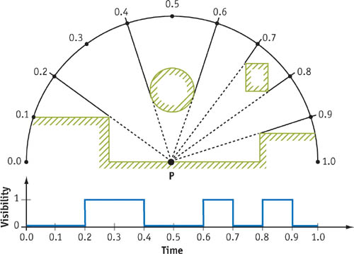
Figure 13-2 A Single Point in the Scene and Its Visibility Function

We now have all we need for precomputed visibility of hard shadows; given a rise vector, a fall vector, and time of day, we can compute the visibility function to determine if the point is in shadow.

In order to turn this into a soft shadow algorithm, we extend the light source along its trajectory. Now instead of computing shadows from a point light source, we compute shadows from a linear light source. Imagine a time interval 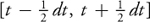. Over this time, the light source will sweep out a curve in space. If we take the average lighting over the time interval 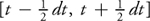, we will have computed the correct shadowing from the linear light source. This means that we can apply the same information used to render a hard shadow image to rendering a soft shadowed image. See Figure 13-3.

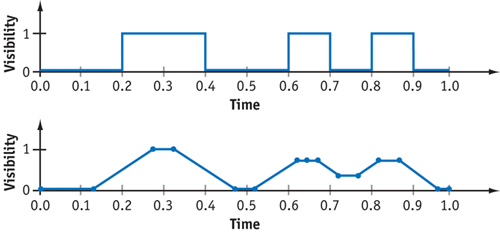
Figure 13-3 The Point Light Visibility Function and Corresponding Linear Light Visibility Function

13.3 Creating the Maps

In order to generate occlusion interval maps, we have to compute the visibility function from every point on the light source trajectory to every pixel in the occlusion interval map. We do this by taking a sequence of evenly spaced points along the curve, tracing a ray from each occlusion interval map pixel to each of these points, and detecting the rising and falling edges of each visibility function. We store rising and falling edge values in eight bits; so 256 rays are enough to completely capture all of the intervals. To reduce the amount of information stored, we do not store rising and falling edges when a point's normal is facing away from the light source. Because back-facing pixels will be dark anyway, this decision will save space and have no effect on the rendered image.

Computing visibility functions can be done by any ray tracer with the right level of programmability. We computed all data for our scene using a custom shader in the mental ray software package. Computing these textures can be time-consuming, because you have to cast 256 rays for every pixel in the occlusion interval map. For the scene in "Last Chance Gas," it took several hours to compute the shadowing for the entire scene.

We store the rise vector and the fall vector in two sets of color textures, each texture having four channels. A "rise" texture stores the beginning of a light interval in each channel, and the matching "fall" texture stores the ends of the light intervals. It will become obvious why we divide the textures up like this when we describe the algorithm for rendering with occlusion interval maps.

To alleviate the extra memory requirements of storing the occlusion interval maps, we compute our maps at half the size of color textures, which reduces the storage requirements by a factor of four. The resolution of occlusion interval maps can be reduced because the softness of the shadows has a blurring effect that makes up for the lower resolution. In some cases, we found that we could even lower the resolution of the maps beyond half the color texture sizes without noticeable artifacts.

For parameterizing the objects, we use the objects' texture coordinates. Because the pixels of the occlusion interval map store information that depends on position, the objects' texture coordinates cannot overlap. For objects with tiled textures, this means computing a new set of unique texture coordinates.

13.4 Rendering

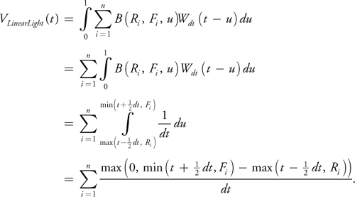
When rendering, we have to average the visibility function over an interval of parameter values. In mathematical terms, this means performing a convolution with a window function of width dt. The equation for this calculation is:

where V_PointLight is the visibility function and W_dt is a box filter of width dt, defined as W_dt (t) = 1/dt for -dt/2 < t < dt/2, and W_dt (t) = 0 otherwise. Given a rise vector R = (R ₁, R ₂,...,R_n ) and a fall vector F = (F ₁, F ₂,...,F_n ), then we can express V_PointLight as:

where B(a, b, t) is the boxcar function, defined as B(a, b, t) = 1 for a < t < b and B(a, b, t) = 0 otherwise. We can now evaluate V_LinearLight as follows:

Using the preceding equation, we can easily calculate soft shadowing for a single rise/fall pair using just min, max, and subtraction. Fortunately, we optimize this even further. Because shader instructions operate on four-component vectors, four intervals can be done simultaneously at the same cost of doing a single interval. This is why we pack the rises and falls into separate textures. The final Cg code is shown in Listing 13-1.

Example 13-1. Function for Computing Soft Shadows Using Occlusion Interval Maps

 half softshadow(sampler2D riseTexture,                 sampler2D fallTexture,                 float2 texCoord,                 half intervalStart,                 half intervalEnd,                 half intervalInverseWidth) {   half4 rise = h4tex2D (riseTexture, texCoord);   half4 fall = h4tex2D (fallTexture, texCoord);   half4 minTerm = min (fall, intervalEnd);   half4 maxTerm = max (rise, intervalStart);   return dot (intervalInverseWidth, saturate (minTerm - maxTerm)); }

Note that saturate(x) is used in place of max(0, x). The two operations will always be equivalent because the quantity being considered is the width of the visible light source interval, which is always less than 1. We choose to use saturate(x) over max(0, x) because it can be applied as an output modifier, saving an instruction. We used the 16-bit half data type and found it perfectly suited to our needs, because our calculations exceeded the range of fixed precision but did not require full 32-bit floating point.

The dot product on the last line of Listing 13-1 is not used for its usual geometric purpose; we use it to simultaneously divide by the light source width and add together the shadow values that are computed in parallel. We pass the values to the shader as intervalStart = t - 1/2dt, intervalEnd = t + 1/2dt, and intervalInverseWidth = 1/dt.

This shader compiles to only six assembly-code instructions for the GeForce FX: two texture lookups, a min, a max, a subtraction with a saturate modifier, and a dot product. The function computes up to four intervals' worth of shadows. If there are multiple rise and fall textures, we just call the function multiple times and add the results together.

13.5 Limitations

As previously discussed, the technique works only for static scenes with a single light traveling on a fixed trajectory. This means it would not work for shadowing on characters and other dynamic objects, but it is well suited for shadowing in static outdoor environments.

Because occlusion interval maps require all eight bits of precision per channel, texture compression will result in visual artifacts. Thus, texture compression has to be disabled, resulting in increased texture usage. This increase is offset by the lower resolution of the occlusion interval maps. The discontinuities in the occlusion interval maps mean that bilinear filtering produced artifacts as well. As a result, any kind of texture filtering must also be disabled on occlusion interval maps. This gives the shadows a blocky look. Once again, because of the smoothness of the shadowing, this effect is not as noticeable as it would be on detailed color textures.

Another visual artifact comes from the fact that the Sun is approximated by a linear light source. If you look closely at the shadow boundaries, you will see that shadows are smoother in the direction parallel to the light source path and harder in the perpendicular direction. Fortunately, this effect is subtle unless the light source is very large. For the range of widths we used, the effect is not very noticeable. Heidrich et al. (2000) also used linear lights to approximate area lights and noted that the shadowing from a linear light source looks very much like the shadowing from a true area light source. See Figure 13-4.

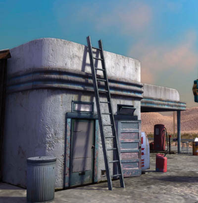
Figure 13-4 Lighting a Ladder

13.6 Conclusion

Rendering soft shadows in real time is an extremely difficult problem. Figures 13-5 and 13-6 show two examples of the subtleties involved. Precomputed visibility techniques produce soft shadows by imposing assumptions on the scene and on the light source. In the case of occlusion interval maps, we trade generality for performance to obtain a soft shadow algorithm that runs in real time on static scenes. Occlusion interval maps can act as a replacement for static light maps, allowing dynamic effects such as the variation of lighting from sunrise to sunset, as in "Last Chance Gas."

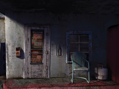
Figure 13-5 The Gas Station Entrance

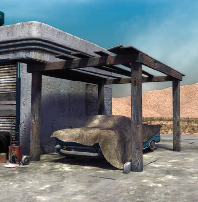
Figure 13-6 Shadows on the Car's Tarp

13.7 References

We also considered using the soft shadow volume technique presented by Assarsson et al., but we had too much geometry in our scene for a shadow volume technique to remain real-time.

Assarsson, Ulf, Michael Dougherty, Michael Mounier, and Tomas Akenine-Möller. 2003. "An Optimized Soft Shadow Volume Algorithm with Real-Time Performance." Graphics Hardware, pp. 33–40.

Heidrich, Wolfgang, Stefan Brabec, and Hans-Peter Seidel. 2000. "Soft Shadow Maps for Linear Lights." In 11th Eurographics Workshop on Rendering, pp. 269–280.

Max, N. L. 1988. "Horizon Mapping: Shadows for Bump-Mapped Surfaces. The Visual Computer 4(2), pp. 109–117.

Sloan, Peter-Pike, Jan Kautz, and John Snyder. 2002. "Precomputed Radiance Transfer for Real-Time Rendering in Dynamic, Low-Frequency Lighting Environments." ACM Transactions on Graphics 21, pp. 527–536.

Copyright

Many of the designations used by manufacturers and sellers to distinguish their products are claimed as trademarks. Where those designations appear in this book, and Addison-Wesley was aware of a trademark claim, the designations have been printed with initial capital letters or in all capitals.

The authors and publisher have taken care in the preparation of this book, but make no expressed or implied warranty of any kind and assume no responsibility for errors or omissions. No liability is assumed for incidental or consequential damages in connection with or arising out of the use of the information or programs contained herein.

The publisher offers discounts on this book when ordered in quantity for bulk purchases and special sales. For more information, please contact:

U.S. Corporate and Government Sales
(800) 382-3419
corpsales@pearsontechgroup.com

For sales outside of the U.S., please contact:

International Sales
international@pearsoned.com

Visit Addison-Wesley on the Web: www.awprofessional.com

Library of Congress Control Number: 2004100582

GeForce™ and NVIDIA Quadro^® are trademarks or registered trademarks of NVIDIA Corporation.
RenderMan^® is a registered trademark of Pixar Animation Studios.
"Shadow Map Antialiasing" © 2003 NVIDIA Corporation and Pixar Animation Studios.
"Cinematic Lighting" © 2003 Pixar Animation Studios.
Dawn images © 2002 NVIDIA Corporation. Vulcan images © 2003 NVIDIA Corporation.

All rights reserved. No part of this publication may be reproduced, stored in a retrieval system, or transmitted, in any form, or by any means, electronic, mechanical, photocopying, recording, or otherwise, without the prior consent of the publisher. Printed in the United States of America. Published simultaneously in Canada.

For information on obtaining permission for use of material from this work, please submit a written request to:

Pearson Education, Inc.
Rights and Contracts Department
One Lake Street
Upper Saddle River, NJ 07458

Text printed on recycled and acid-free paper.

5 6 7 8 9 10 QWT 09 08 07

5th Printing September 2007

Part II: Lighting and Shadows

Part III: Materials

Part IV: Image Processing

Part V: Performance and Practicalities

Part VI: Beyond Triangles

Preface