GPU Gems

GPU Gems is now available, right here, online. You can purchase a beautifully printed version of this book, and others in the series, at a 30% discount courtesy of InformIT and Addison-Wesley.

The CD content, including demos and content, is available on the web and for download.

Chapter 39. Volume Rendering Techniques

Milan Ikits
University of Utah

Joe Kniss
University of Utah

Aaron Lefohn
University of California, Davis

Charles Hansen
University of Utah

This chapter presents texture-based volume rendering techniques that are used for visualizing three-dimensional data sets and for creating high-quality special effects.

39.1 Introduction

Many visual effects are volumetric in nature. Fluids, clouds, fire, smoke, fog, and dust are difficult to model with geometric primitives. Volumetric models are better suited for creating such effects. These models assume that light is emitted, absorbed, and scattered by a large number of particles in the volume. See Figure 39-1 for two examples.

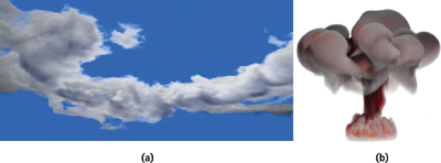
Figure 39-1 Volumetric Effects

In addition to modeling and rendering volumetric phenomena, volume rendering is essential to scientific and engineering applications that require visualization of three-dimensional data sets. Examples include visualization of data acquired by medical imaging devices or resulting from computational fluid dynamics simulations. Users of interactive volume rendering applications rely on the performance of modern graphics accelerators for efficient data exploration and feature discovery.

This chapter describes volume rendering techniques that exploit the flexible programming model and 3D texturing capabilities of modern GPUs. Although it is possible to implement other popular volume rendering algorithms on the GPU, such as ray casting (Roettger et al. 2003, Krüger and Westermann 2003), this chapter describes texture-based volume rendering only. Texture-based techniques are easily combined with polygonal algorithms, require only a few render passes, and offer a great level of interactivity without sacrificing the quality of rendering.

Section 39.2 introduces the terminology and explains the process of direct volume rendering. Section 39.3 describes the components of a typical texture-based volume rendering application, and illustrates it with a simple example. Section 39.4 provides additional implementation details, which expand the capabilities of the basic volume renderer. Section 39.5 describes advanced techniques for incorporating more realistic lighting effects and adding procedural details to the rendering. Section 39.6 concludes with a summary of relevant performance considerations.

39.2 Volume Rendering

Direct volume rendering methods generate images of a 3D volumetric data set without explicitly extracting geometric surfaces from the data (Levoy 1988). These techniques use an optical model to map data values to optical properties, such as color and opacity (Max 1995). During rendering, optical properties are accumulated along each viewing ray to form an image of the data (see Figure 39-2).

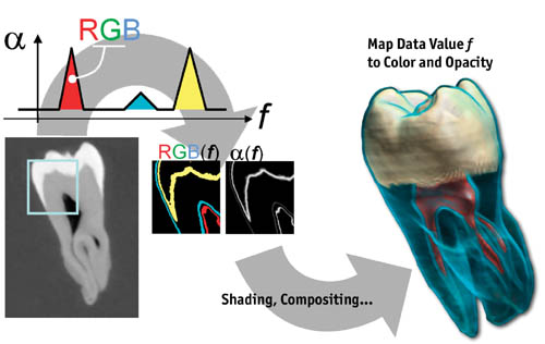
Figure 39-2 The Process of Volume Rendering

Although the data set is interpreted as a continuous function in space, for practical purposes it is represented by a uniform 3D array of samples. In graphics memory, volume data is stored as a stack of 2D texture slices or as a single 3D texture object. The term voxel denotes an individual "volume element," similar to the terms pixel for "picture element" and texel for "texture element." Each voxel corresponds to a location in data space and has one or more data values associated with it. Values at intermediate locations are obtained by interpolating data at neighboring volume elements. This process is known as reconstruction and plays an important role in volume rendering and processing applications.

In essence, the role of the optical model is to describe how particles in the volume interact with light. For example, the most commonly used model assumes that the volume consists of particles that simultaneously emit and absorb light. More complex models incorporate local illumination and volumetric shadows, and they account for light scattering effects. Optical parameters are specified by the data values directly, or they are computed from applying one or more transfer functions to the data. The goal of the transfer function in visualization applications is to emphasize or classify features of interest in the data. Typically, transfer functions are implemented by texture lookup tables, though simple functions can also be computed in the fragment shader. For example, Figure 39-2 illustrates the use of a transfer function to extract material boundaries from a CT scan of a tooth.

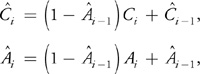
Images are created by sampling the volume along all viewing rays and accumulating the resulting optical properties, as shown in Figure 39-3. For the emission-absorption model, the accumulated color and opacity are computed according to Equation 1, where C_i and A_i are the color and opacity assigned by the transfer function to the data value at sample i.

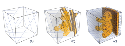
Figure 39-3 Volume Sampling and Compositing

Equation 1 Discrete Volume Rendering Equations

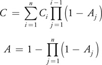
Opacity A_i approximates the absorption, and opacity-weighted color C_i approximates the emission and the absorption along the ray segment between samples i and i+ 1. For the color component, the product in the sum represents the amount by which the light emitted at sample i is attenuated before reaching the eye. This formula is efficiently evaluated by sorting the samples along the viewing ray and computing the accumulated color C and opacity A iteratively. Section 39.4 describes how the compositing step can be performed via alpha blending. Because Equation 1 is a numerical approximation to the continuous optical model, the sampling rate s, which is inversely proportional to the distance between the samples l, greatly influences the accuracy of approximation and the quality of rendering.

Texture-based volume rendering techniques perform the sampling and compositing steps by rendering a set of 2D geometric primitives inside the volume, as shown in Figure 39-3. Each primitive is assigned texture coordinates for sampling the volume texture. The proxy geometry is rasterized and blended into the frame buffer in back-to-front or front-to-back order. In the fragment shading stage, the interpolated texture coordinates are used for a data texture lookup. Next, the interpolated data values act as texture coordinates for a dependent lookup into the transfer function textures. Illumination techniques may modify the resulting color before it is sent to the compositing stage of the pipeline.

39.3 Texture-Based Volume Rendering

In general, as shown in Figure 39-4, texture-based volume rendering algorithms can be divided into three stages: (1) Initialize, (2) Update, and (3) Draw. The Initialize stage is usually performed only once. The Update and Draw stages are executed whenever the application receives user input—for example, when viewing or rendering parameters change.

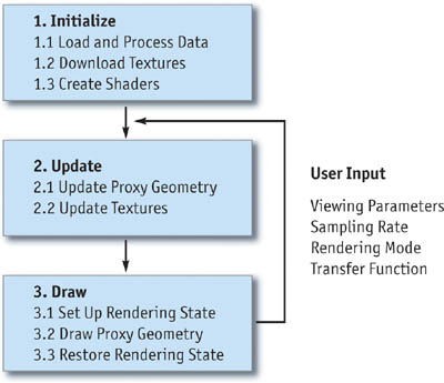
Figure 39-4 The Steps of a Typical Texture-Based Volume Rendering Implementation

At the beginning of the application, data volumes are loaded into CPU memory. In certain cases, the data sets also need to be processed before packing and downloading them to texture memory. For example, one may choose to compute gradients or down-sample the data at this stage. Some of the data processing operations can also be done outside the application. Transfer function lookup tables and fragment shaders are typically created in the Initialize stage of the application.

After initialization and every time viewing parameters change, the proxy geometry is computed and stored in vertex arrays. When the data set is stored as a 3D texture object, the proxy geometry consists of a set of polygons, slicing through the volume perpendicular to the viewing direction (see Section 39.4.2). Slice polygons are computed by first intersecting the slicing planes with the edges of the volume bounding box and then sorting the resulting vertices in a clockwise or counterclockwise direction around their center. For each vertex, the corresponding 3D texture coordinate is calculated on the CPU, in a vertex program, or via automatic texture-coordinate generation.

When a data set is stored as a set of 2D texture slices, the proxy polygons are simply rectangles aligned with the slices. Despite being faster, this approach has several disadvantages. First, it requires three times more memory, because the data slices need to be replicated along each principal direction. Data replication can be avoided with some performance overhead by reconstructing slices on the fly (Lefohn et al. 2004). Second, the sampling rate depends on the resolution of the volume. This problem can be solved by adding intermediate slices and performing trilinear interpolation with a fragment shader (Rezk-Salama et al. 2000). Third, the sampling distance changes with the viewpoint, resulting in intensity variations as the camera moves and image-popping artifacts when switching from one set of slices to another (Kniss et al. 2002b).

During the Update stage, textures are refreshed if the rendering mode or the transfer function parameters change. Also, opacity correction of the transfer function textures is performed if the sampling rate has changed (see Equation 3).

Before the slice polygons are drawn in sorted order, the rendering state needs to be set up appropriately. This step typically includes disabling lighting and culling, and setting up alpha blending. To blend in opaque geometry, depth testing has to be enabled, and writing to the depth buffer has to be disabled. Volume and transfer function textures have to be bound to texture units, which the fragment shader uses for input. At this point, shader input parameters are specified, and vertex arrays are set up for rendering. Finally, after the slices are drawn in sorted order, the rendering state is restored, so that the algorithm does not affect the display of other objects in the scene.

39.3.1 A Simple Example

The following example is intended as a starting point for understanding the implementation details of texture-based volume rendering. In this example, the transfer function is fixed, the data set represents the opacity directly, and the emissive color is set to constant gray. In addition, the viewing direction points along the z axis of the data coordinate frame; therefore, the proxy geometry consists of rectangles in the x-y plane placed uniformly along the z axis. The algorithm consists of the steps shown in Algorithm 39-1.

Example 39-1. The Steps of the Simple Volume Rendering Application

Create and download the data set as a 3D alpha texture.
Load the fragment program shown in Listing 39-1.
Load the modelview and projection matrices.
Enable alpha blending using 1 for the source fragment and (1 – source alpha) for the destination fragment.
Disable lighting and depth testing (there is no opaque geometry in this example).
Bind the data texture to texture unit 0.
Enable and bind the fragment program and specify its input.
Draw textured quads along the z axis. The x-y vertex coordinates are (–1, –1), (1, –1), (1, 1), (–1, 1). The corresponding x-y texture coordinates are (0, 0), (1, 0), (1, 1), (0, 1). The z vertex and texture coordinates increase uniformly from –1 to 1 and 0 to 1, respectively.

Example 39-1. The Fragment Program for the Simple Volume Renderer

 void main(uniform float3 emissiveColor,           uniform sampler3D dataTex,           float3 texCoord : TEXCOORD0,           float4 color : COLOR) {   float a = tex3D(texCoord, dataTex);  // Read 3D data texture   color = a * emissiveColor;           // Multiply color by opacity }

Figure 39-5 shows the image generated by the simple volume renderer. The following sections demonstrate how to make each stage of the example more general and useful for a variety of tasks.

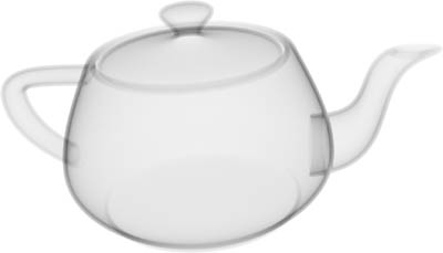
Figure 39-5 Output of the Simple Volume Renderer Using a Voxelized Model of a Familiar Object

39.4 Implementation Details

This section presents an overview of the components commonly used in texture-based volume rendering applications. The goal is to provide enough details to make it easier to understand typical implementations of volume renderers that utilize current-generation consumer graphics hardware, such as the GeForce FX family of cards.

39.4.1 Data Representation and Processing

Volumetric data sets come in a variety of sizes and types. For volume rendering, data is stored in memory in a suitable format, so it can be easily downloaded to graphics memory as textures. Usually, the volume is stored in a single 3D array. Depending on the kind of proxy geometry used, either a single 3D texture object or one to three sets of 2D texture slices are created. The developer also has to choose which available texture formats to use for rendering. For example, power-of-two-size textures are typically used to maximize rendering performance. Frequently, the data set is not in the right format and not the right size, and it may not fit into the available texture memory on the GPU. In simple implementations, data processing is performed in a separate step outside the renderer. In more complex scenarios, data processing becomes an integral part of the application, such as when data values are generated on the fly or when images are created directly from raw data.

To change the size of a data set, one can resample it into a coarser or a finer grid, or pad it at the boundaries. Padding is accomplished by placing the data into a larger volume and filling the empty regions with values. Resampling requires probing the volume (that is, computing interpolated data values at a location from voxel neighbors). Although the commonly used trilinear interpolation technique is easy to implement, it is not always the best choice for resampling, because it can introduce visual artifacts. If the quality of resampling is crucial for the application, more complex interpolation functions are required, such as piecewise cubic polynomials. Fortunately, such operations are easily performed with the help of publicly available toolkits. For example, the Teem toolkit includes a great variety of data-processing tools accessible directly from the command line, exposing the functionality of the underlying libraries without having to write any code (Kindlmann 2003). Examples of using Teem for volume data processing are included on the book's CD and Web site. Advanced data processing can also be performed on the GPU, for example, to create high-quality images (Hadwiger et al. 2001).

Local illumination techniques and multidimensional transfer functions use gradient information during rendering. Most implementations use central differences to obtain the gradient vector at each voxel. The method of central differences approximates the gradient as the difference of data values of two voxel neighbors along a coordinate axis, divided by the physical distance. For example, the following formula computes the x component of the gradient vector at voxel location

Equation 2 Gradient Computation Using Central Differences

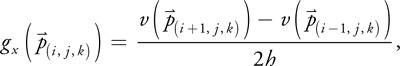
where h is the distance between the voxels along the x axis. To obtain the gradient at data boundaries, the volume is padded by repeating boundary values. Visual artifacts caused by central differences are similar to those resulting from resampling with trilinear interpolation. If visual quality is of concern, more complex derivative functions are needed, such as the ones that Teem provides. Depending on the texture format used, the computed gradients may need to be quantized, scaled, and biased to fit into the available range of values.

Transfer functions emphasize regions in the volume by assigning color and opacity to data values. Histograms are useful for analyzing which ranges of values are important in the data. In general, histograms show the distribution of data values and other related data measures. A 1D histogram is created by dividing up the value range into a number of bins. Each bin contains the number of voxels within the lower and upper bounds assigned to the bin. By examining the histogram, one can see which values are frequent in the data. Histograms, however, do not show the spatial distribution of the samples in the volume.

The output of the data-processing step is a set of textures that are downloaded to the GPU in a later stage. It is sometimes more efficient to combine several textures into a single texture. For example, to reduce the cost of texture lookup and interpolation, the value and normalized gradient textures are usually stored and used together in a single RGBA texture.

39.4.2 Proxy Geometry

During the rendering stage, images of the volume are created by drawing the proxy geometry in sorted order. When the data set is stored in a 3D texture, view-aligned planes are used for slicing the bounding box, resulting in a set of polygons for sampling the volume. Algorithm 39-2 computes the proxy geometry in view space by using the modelview matrix for transforming vertices between the object and view coordinate systems. Proxy polygons are tessellated into triangles, and the resulting vertices are stored in a vertex array for more efficient rendering.

Figure 39-6 illustrates Algorithm 39-2 with two slice polygons. The first polygon contains three vertices, the second is composed of six vertices and is tessellated into six triangles.

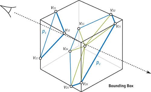
Figure 39-6 View-Aligned Slicing with Two Sampling Planes

There are several ways to generate texture coordinates for the polygon vertices. For example, texture coordinates can be computed on the CPU in step 3(c) of Algorithm 39-2 from the computed vertex positions and the volume bounding box. In this case the coordinates are sent down to GPU memory in a separate vertex array or interleaved with the vertex data. There are different methods for computing the texture coordinates on the GPU, including automatic texture coordinate generation, the texture matrix, or with a vertex program.

Advanced algorithms, such as the one described in Section 39.5, may use a different slicing axis than the viewing direction. In this case, the algorithm works the same way, but the modelview matrix needs to be modified accordingly.

Example 39-2. View-Aligned Slicing for Volume Rendering

Transform the volume bounding box vertices into view coordinates using the modelview matrix.
Find the minimum and maximum z coordinates of the transformed vertices. Compute the number of sampling planes used between these two values using equidistant spacing from the view origin. The sampling distance is computed from the voxel size and current sampling rate.
For each plane in front-to-back or back-to-front order:
1. Test for intersections with the edges of the bounding box. Add each intersection point to a temporary vertex list. Up to six intersections are generated, so the maximum size of the list is fixed.
2. Compute the center of the proxy polygon by averaging the intersection points. Sort the polygon vertices clockwise or counterclockwise by projecting them onto the x-y plane and computing their angle around the center, with the first vertex or the x axis as the reference. Note that to avoid trigonometric computations, the tangent of the angle and the sign of the coordinates, combined into a single scalar value called the pseudo-angle, can be used for sorting the vertices (Moret and Shapiro 1991).
3. Tessellate the proxy polygon into triangles and add the resulting vertices to the output vertex array. The slice polygon can be tessellated into a triangle strip or a triangle fan using the center. Depending on the rendering algorithm, the vertices may need to be transformed back to object space during this step.

39.4.3 Rendering

Transfer Functions

The role of the transfer function is to emphasize features in the data by mapping values and other data measures to optical properties. The simplest and most widely used transfer functions are one dimensional, and they map the range of data values to color and opacity. Typically, these transfer functions are implemented with 1D texture lookup tables. When the lookup table is built, color and opacity are usually assigned separately by the transfer function. For correct rendering, the color components need to be multiplied by the opacity, because the color approximates both the emission and the absorption within a ray segment (opacity-weighted color)(Wittenbrink et al. 1998).

Example 39-2. The Fragment Program for 1D Transfer Function Dependent Textures

 void main(uniform sampler3D dataTex,           uniform sampler1D tfTex,           float3 texCoord : TEXCOORD0,           float4 color : COLOR) {   float v = tex3d(texCoord, dataTex);  // Read 3D data texture and   color = tex1d(v, tfTex);             // transfer function texture }

Using data value as the only measure for controlling the assignment of color and opacity may limit the effectiveness of classifying features in the data. Incorporating other data measures into the transfer function, such as gradient magnitude, allows for finer control and more sophisticated visualization (Kindlmann and Durkin 1998, Kindlmann 1999). For example, see Figure 39-7 for an illustration of the difference between using one- and two-dimensional transfer functions based on the data value and the gradient magnitude.

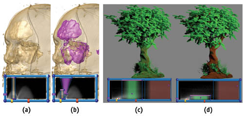
Figure 39-7 The Difference Between 1D and 2D Transfer Functions

Transfer function design is a difficult iterative procedure that requires significant insight into the underlying data set. Some information is provided by the histogram of data values, indicating which ranges of values should be emphasized. The user interface is an important component of the interactive design procedure. Typically, the interface consists of a 1D curve editor for specifying transfer functions via a set of control points. Another approach is to use direct manipulation widgets for painting directly into the transfer function texture (Kniss et al. 2002a). The lower portions of the images in Figure 39-7 illustrate the latter technique. The widgets provide a view of the joint distribution of data values, represented by the horizontal axis, and gradient magnitudes, represented by the vertical axis. Arches within the value and gradient magnitude distribution indicate the presence of material boundaries. A set of brushes is provided for painting into the 2D transfer function dependent texture, which assigns the resulting color and opacity to voxels with the corresponding ranges of data values and gradient magnitudes.

The assigned opacity also depends on the sampling rate. For example, when using fewer slices, the opacity has to be scaled up, so that the overall intensity of the image remains the same. Equation 3 is used for correcting the transfer function opacity whenever the user changes the sampling rate s from the reference sampling rate s ₀:

Equation 3 Formula for Opacity Correction

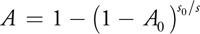
To control the quality and speed of rendering, users typically change the maximum number of slices, or the relative sampling rate s/s ₀, via the user interface.

Illumination

Illumination models are used for improving the visual appearance of objects. Simple models locally approximate the light intensity reflected from the surface of an object. The most common approximation is the Blinn-Phong model, which computes the reflected intensity as a function of local surface normal , the direction , and intensity I_L of the point light source, and ambient, diffuse, specular, and shininess coefficients k_a , k_d , k_s , and n:

Equation 4 The Blinn-Phong Model for Local Illumination

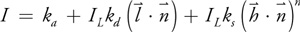
The computed intensity is used to modulate the color components from the transfer function. Typically, Equation 4 is evaluated in the fragment shader, requiring per-pixel normal information. In volume rendering applications, the normalized gradient vector is used as the surface normal. Unfortunately, the gradient is not well defined in homogeneous regions of the volume. For volume rendering, the Blinn-Phong model is frequently modified, so that only those regions with high gradient magnitudes are shaded (Kniss et al. 2002b).

Local illumination ignores indirect light contributions, shadows, and other global effects, as illustrated by Figure 39-8. Section 39.5 describes how to incorporate simple global illumination models into the rendering model for creating high-quality volumetric effects.

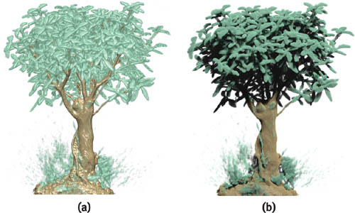
Figure 39-8 Comparison of Simple and Complex Lighting Effects

Compositing

To efficiently evaluate the volume rendering equation (Equation 1), samples are sorted in back-to-front order, and the accumulated color and opacity are computed iteratively. A single step of the compositing process is known as the Over operator:

Equation 5 Back-to-Front Compositing Equations

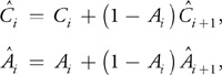
where C_i and A_i are the color and opacity obtained from the fragment shading stage for segment i along the viewing ray, and is the accumulated color from the back of the volume. If samples are sorted in front-to-back order, the Under operator is used:

Equation 6 Front-to-Back Compositing Equations

where and are the accumulated color and opacity from the front of the volume.

The compositing equations (Equations 5 and 6) are easily implemented with hardware alpha blending. For the Over operator, the source blending factor is set to 1 and the destination blending factor is set to (1 – source alpha). For the Under operator, the source blending factor is set to (1 – destination alpha) and the destination factor is set to 1. Alternatively, if the hardware allows for reading and writing the same buffer, compositing can be performed in the fragment shading stage by projecting the proxy polygon vertices onto the viewport rectangle (see Section 39.5).

To blend opaque geometry into the volume, the geometry needs to be drawn before the volume, because the depth test will cull proxy fragments that are inside objects. The Under operator requires drawing the geometry and the volume into separate color buffers that are composited at the end. In this case, the depth values from the geometry pass are used for culling fragments in the volume rendering pass.

39.5 Advanced Techniques

This section describes techniques for improving the quality of rendering and creating volumetric special effects.

39.5.1 Volumetric Lighting

The local illumination model presented in the previous section adds important visual cues to the rendering. Such a simple model is unrealistic, however, because it assumes that light arrives at a sample without interacting with the rest of the volume. Furthermore, this kind of lighting assumes a surface-based model, which is inappropriate for volumetric materials. One way to incorporate complex lighting effects, such as volumetric shadows, is to precompute a shadow volume for storing the amount of light arriving at each sample after being attenuated by the intervening material. During rendering, the interpolated values from this volumetric shadow map are multiplied by colors from the transfer function. But in addition to using extra memory, volumetric shadow maps result in visual artifacts such as blurry shadows and dark images.

A better alternative is to use a pixel buffer to accumulate the amount of light attenuated from the light's point of view (Kniss et al. 2003). To do this efficiently, the slicing axis is set halfway between the view and the light directions, as shown in Figure 39-9a. This allows the same slice to be rendered from both the eye and the light points of view. The amount of light arriving at a particular slice is equal to 1 minus the accumulated opacity of the previously rendered slices. Each slice is first rendered from the eye's point of view, using the results of the previous pass rendered from the light's point of view, which are used to modulate the brightness of samples in the current slice. The same slice is then rendered from the light's point of view to calculate the intensity of the light arriving at the next slice. Algorithm 39-3 uses two buffers: one for the eye and one for the light. Figure 39-10 shows the setup described in Algorithm 39-3.

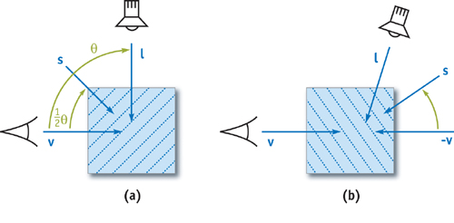
Figure 39-9 Half-Angle Slicing for Incremental Lighting Computations

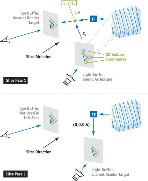
Figure 39-10 Two-Pass Volumetric Shadow Setup

Example 39-3. Two-Pass Volume Rendering with Shadows

Clear the eye buffer and initialize the light buffer to the light color C_L . A texture map can be used to initialize the light buffer for creating special effects, such as spotlights.
Compute the proxy geometry in object space using Algorithm 39-1. When the dot product of the light and the view directions is positive, set the slice direction to halfway between the light and the view directions, as shown in Figure 39-9a. In this case, the volume is rendered front to back for the eye using the Under operator (see Section 39.4.3). When the dot product is negative, slice along the vector halfway between the light and the inverted view directions, and render the volume back to front for the eye using the Over operator (see Figure 39-9b). In both cases, render the volume front to back for the light using the Over operator.
For each slice:
1. Pass 1: Render and blend the slice into the eye buffer.
  1. Project the slice vertices to the light buffer using the light's modelview and projection matrices. Convert the resulting vertex positions to 2D texture coordinates based on the size of the light's viewport and the light buffer.
  2. Bind the light buffer as a texture to an available texture unit and use the texture coordinates computed in step 3(a)(i). Recall that a set of 3D texture coordinates is also needed for the data texture lookup.
  3. In the fragment shader, evaluate the transfer function for reflective color C and opacity A. Next, multiply C by the color from the light buffer C_L , and blend C and A into the eye buffer using the appropriate operator for the current slice direction.
2. Pass 2: Render and blend the slice into the light buffer using the Over operator. In the fragment shader, evaluate the transfer function for the alpha component and set the fragment color to 0.

Volumetric shadows greatly improve the realism of rendered scenes, as shown in Figure 39-11. Note that as the angle between the observer and the light directions changes, the slice distance needs to be adjusted to maintain a constant sampling rate. If the desired sampling distance along the observer view direction is d_v and the angle between the observer and the light view directions is , the slice spacing d_s is given by Equation 7:

Equation 7 Relationship Between Slice Spacing and Sampling Distance Used for Half-Angle Slicing

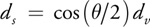
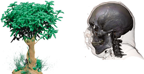
Figure 39-11 Examples of Volume Rendering with Shadows

Unfortunately, Algorithm 39-3 still produces dark and unrealistic images, because it ignores contributions from light scattering within the volume. Scattering effects can be fully captured through physically based volume lighting models, which are too complex for interactive rendering. It is possible, however, to extend Algorithm 39-3 to approximate certain scattering phenomena. One such phenomenon is translucency, which is the result of light propagating into and scattering throughout a material. While general scattering computations consider the incoming light from all directions, for translucency it is sufficient to include the incoming light within a cone in the direction of the light source only, as shown in Figure 39-12. The result of this simplification is that the indirect scattering contribution at a particular sample depends on a local neighborhood of samples computed in the previous iteration of Algorithm 39-3. Thus, translucency effects are possible to incorporate by propagating and blurring indirect lighting components from slice to slice in the volume.

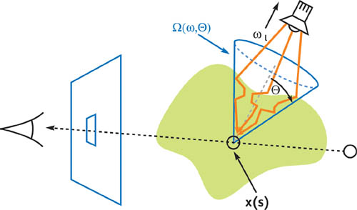
Figure 39-12 Setup for the Translucency Approximation

To incorporate translucency into Algorithm 39-3, first add indirect attenuation parameters A_i . These parameters are alpha values for each of the RGB color channels, as opposed to the single alpha value A used in Algorithm 39-3. Second, instead of initializing the light buffer with the light color C_L , use 1 - C_L . Third, in step 3(a)(iii), multiply C by 1 - A_i , that is, 1 minus the color value read from the light buffer. In step 3(b), set the color in the fragment shader to A_i instead of 0, and replace the Over operator with the following blending operation:

Equation 8 Light Buffer Compositing for the Translucency Model

In Equation 8, C ₁ is the color of the incoming fragment, and C ₀ is the color currently in the target render buffer.

Next, an additional buffer is used to blur the indirect attenuation components when updating the contents of the light buffer in step 3(b). The two buffers are used in an alternating fashion, such that the current light buffer is sampled once in step 3(a) for the eye, and multiple times in step 3(b) for the light. The next light buffer is the render target in step 3(b). This relationship changes after each slice, so the next buffer becomes the current buffer and vice versa.

To sample the indirect components for the blur operation, the texture coordinates for the current light buffer, in all but one texture unit, are modified using a perturbation texture. The radius of the blur circle, used to scale the perturbations, is given by a user-defined blur angle and the sample distance d:

Equation 9 Blur Radius for the Translucency Approximation

In the fragment shader during step 3(b), the current light buffer is read using the modified texture coordinates. The blurred attenuation is computed as a weighted sum of the values read from the light buffer, and then blended into the next light buffer.

Figure 39-13 shows an example of translucent volume rendering using a fish CT data set. This technique is important for creating convincing images of clouds and other atmospheric phenomena (see Figures 39-1 and 39-14a). Because a separate opacity for each color component is used in step 3(b), it is possible to control the amount of light penetrating into a region by modifying the A_i values to be smaller or larger than the alpha value A used in step 3(a). When the A_i values are less than A, light penetrates deeply into the volume, even if from the eye's point of view, the material appears optically dense. Also, because an independent alpha is specified for each color channel, light changes color as it penetrates deeper into the volume. This is much like the effect of holding a flashlight under your hand: the light enters white and exits red. This effect is achieved by making the A_i value for red smaller than the A_i values for green and blue, resulting in a lower attenuation of the red component than the green and blue components.

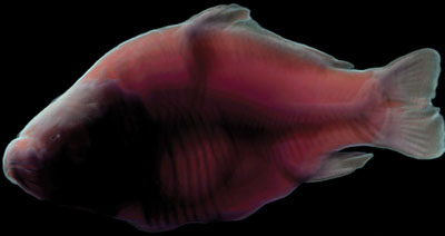
Figure 39-13 Example of Volume Rendering with Translucent Materials

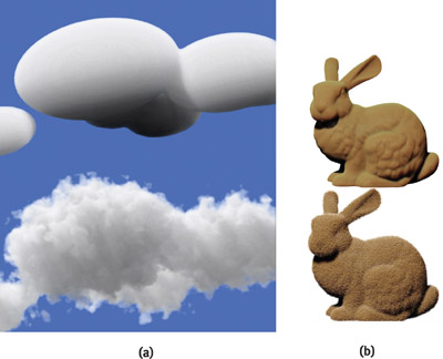
Figure 39-14 Examples of the Volume Perturbation Technique

Computing volumetric light transport in screen space, using a 2D buffer, is advantageous for a variety of reasons. Matching the resolutions of light propagation and the viewport produces crisp shadows with minimal aliasing artifacts. The method presented in this subsection decouples the resolution of the light transport from the 3D data grid, and it permits accurate lighting of procedural volumetric texturing effects, as described in the following subsection.

39.5.2 Procedural Rendering

One drawback of volume rendering is that small high-frequency details cannot be represented in low-resolution volumes. High-frequency details are essential for capturing the characteristics of many volumetric phenomena such as clouds, smoke, trees, hair, and fur. Procedural noise simulation is a powerful technique for adding detail to low-resolution volume data (Ebert et al. 2002). The general approach uses a coarse model for the macrostructure and procedural noise for the microstructure. Described next are two ways of adding procedural noise to texture-based volume rendering. The first approach perturbs optical properties in the shading stage; the second method perturbs the volume itself.

Both approaches use a small noise volume. In this volume, each voxel is initialized to four random numbers, stored as RGBA components, and blurred slightly to hide artifacts caused by trilinear interpolation. Multiple copies of the noise texture are used for each slice at different scales during rendering. Per-pixel perturbation is computed as a weighted sum of the individual noise components. To animate the perturbation, a varying offset vector can be added to the noise texture coordinates in the fragment shader.

The first technique uses the four per-pixel noise components to modify optical properties of the volume after the transfer function has been evaluated. This results in materials that appear to have irregularities. By selecting which optical properties to modify, different effects are achieved.

The second method uses noise to modify the location of the data access in the volume (Kniss et al. 2003). In this case, three components of the noise texture form a vector, which is added to the texture coordinates for the data texture lookup. Figure 39-14 illustrates how volume perturbation is used to add intricate detail to coarse volumetric models.

39.6 Performance Considerations

Texture-based volume rendering can easily push the performance limits of modern GPUs. This section covers a few considerations specific to volume rendering on GPUs.

39.6.1 Rasterization Bottlenecks

Unlike most graphics applications, texture-based volume renderers use a small number of relatively large geometric primitives. The rasterizer produces many fragments per primitive, which can easily become the bottleneck in the pipeline. In addition, unlike opaque objects, the transparent proxy geometry used in volume rendering cannot leverage the early depth-culling capabilities of modern GPUs. The rasterization bottleneck is exacerbated by the large number of slices needed to render high-quality images. In addition, the frame buffer contents in the compositing stage have to be read back every time a fragment is processed by the fragment shader or the compositing hardware.

For these reasons, it is important to draw proxy geometry that generates only the required fragments. Simply drawing large quads that cover the volume leads to a very slow implementation. The rasterization pressure is reduced by making the viewport smaller, decreasing the sample rate, using preintegrated classification (Engel et al. 2001), and by not drawing empty regions of the volume (Li et al. 2003, Krüger and Westermann 2003). Empty-space skipping can efficiently balance the available geometry and fragment processing bandwidth.

Fragment Program Limitations

Volume rendering performance is largely influenced by the complexity of the fragment shader. Precomputed lookup tables may be faster than fragment programs with many complex instructions. Dependent texture reads, however, can result in pipeline stalls, significantly reducing rendering speed. Achieving peak performance requires finding the correct balance of fragment operations and texture reads, which can be a challenging profiling task.

Texture Memory Limitations

The trilinear interpolation (quadrilinear when using mipmaps) used in volume rendering requires at least eight texture lookups, making it more expensive than the bilinear (trilinear with mipmaps) interpolation used in standard 2D texture mapping. In addition, when using large 3D textures, the texture caches may not be as efficient at hiding the latency of texture memory access as they are when using 2D textures. When the speed of rendering is critical, smaller textures, texture compression, and lower precision types can reduce the pressure on the texture memory subsystem. Efficient compression schemes have recently emerged that achieve high texture compression ratios without affecting the rendering performance (Schneider and Westermann 2003). Finally, the arithmetic and memory systems in modern GPUs operate on all values in an RGBA tuple simultaneously. Packing data into RGBA tuples increases performance by lessening the bandwidth requirements.

39.7 Summary

Volume rendering is an important graphics and visualization technique. A volume renderer can be used for displaying not only surfaces of a model but also the intricate detail contained within. The first half of this chapter presented a typical implementation of a texture-based volume renderer with view-aligned proxy geometry. In Section 39.5, two advanced techniques built upon the basic implementation were described. The presented techniques improve the quality of images by adding volumetric shadows, translucency effects, and random detail to the standard rendering model.

Volume rendering has been around for over a decade and is still an active area of graphics and visualization research. Interested readers are referred to the list of references for further details and state-of-the-art techniques.

39.8 References

Ebert, D., F. Musgrave, D. Peachey, K. Perlin, S. Worley, W. Mark, and J. Hart. 2002. Texturing and Modeling: A Procedural Approach. Morgan Kaufmann.

Engel, K., M. Kraus, and T. Ertl. 2001. "High-Quality Pre-Integrated Volume Rendering Using Hardware-Accelerated Pixel Shading." In Proceedings of the SIGGRAPH/Eurographics Workshop on Graphics Hardware 2001, pp. 9–16.

Hadwiger, M., T. Teußl, H. Hauser, and E. Gröller. 2001 "Hardware-Accelerated High-Quality Filtering on PC Hardware." In Proceedings of the International Workshop on Vision, Modeling, and Visualization 2001, pp. 105–112.

Kindlmann, G., and J. Durkin. 1998. "Semi-Automatic Generation of Transfer Functions for Direct Volume Rendering." In Proceedings of the IEEE Symposium on Volume Visualization, pp. 79–86.

Kindlmann, G. 1999. "Semi-Automatic Generation of Transfer Functions for Direct Volume Rendering." Master's Thesis, Department of Computer Science, Cornell University.

Kindlmann, G. 2003. The Teem Toolkit. http://teem.sourceforge.net

Kniss, J., G. Kindlmann, and C. Hansen. 2002a. "Multidimensional Transfer Functions for Interactive Volume Rendering." IEEE Transactions on Visualization and Computer Graphics 8(4), pp. 270–285.

Kniss, J., K. Engel, M. Hadwiger, and C. Rezk-Salama. 2002b. "High-Quality Volume Graphics on Consumer PC Hardware." Course 42, ACM SIGGRAPH.

Kniss, J., S. Premo e, C. Hansen, P. Shirley, and A. McPherson. 2003. "A Model for Volume Lighting and Modeling." IEEE Transactions on Visualization and Computer Graphics 9(2), pp. 150–162.

Krüger, J., and R. Westermann. 2003. "Acceleration Techniques for GPU-Based Volume Rendering." In Proceedings of IEEE Visualization, pp. 287–292.

Lefohn, A., J. Kniss, C. Hansen, and R. Whitaker. 2004. "A Streaming Narrow-Band Algorithm: Interactive Deformation and Visualization of Level Sets." IEEE Transactions on Visualization and Computer Graphics (to appear).

Levoy, M. 1988. "Display of Surfaces from Volume Data." IEEE Computer Graphics & Applications 8(2), pp. 29–37.

Li, W., K. Mueller, and A. Kaufman. 2003. "Empty Space Skipping and Occlusion Clipping for Texture-Based Volume Rendering." In Proceedings of IEEE Visualization, pp. 317–324.

Max, N. 1995. "Optical Models for Direct Volume Rendering." IEEE Transactions on Visualization and Computer Graphics 1(2), pp. 97–108.

Moret, B., and H. Shapiro. 1991. Algorithms from P to NP. Benjamin Cummings.

Rezk-Salama, C., K. Engel, M. Bauer, G. Greiner, and T. Ertl. 2000. "Interactive Volume Rendering on Standard PC Graphics Hardware Using Multi-Textures and Multi-Stage Rasterization." In Proceedings of the SIGGRAPH/Eurographics Workshop on Graphics Hardware 2000, pp. 109–118.

Roettger, S., S. Guthe, D. Weiskopf, T. Ertl, and W. Strasser. 2003. "Smart Hardware-Accelerated Volume Rendering." In Proceedings of the Eurographics/IEEE TVCG Symposium on Visualization, pp. 231–238.

Schneider, J., and R. Westermann. 2003. "Compression Domain Volume Rendering." In Proceedings of IEEE Visualization, pp. 293–300.

Weiskopf, D., K. Engel, M. Hadwiger, J. Kniss, and A. Lefohn. 2003. "Interactive Visualization of Volumetric Data on Consumer PC Hardware." Tutorial 1. IEEE Visualization.

Wittenbrink, C., T. Malzbender, and M. Goss. 1998. "Opacity-Weighted Color Interpolation for Volume Sampling." In Proceedings of the IEEE Symposium on Volume Visualization, pp. 135–142.

Copyright

Many of the designations used by manufacturers and sellers to distinguish their products are claimed as trademarks. Where those designations appear in this book, and Addison-Wesley was aware of a trademark claim, the designations have been printed with initial capital letters or in all capitals.

The authors and publisher have taken care in the preparation of this book, but make no expressed or implied warranty of any kind and assume no responsibility for errors or omissions. No liability is assumed for incidental or consequential damages in connection with or arising out of the use of the information or programs contained herein.

The publisher offers discounts on this book when ordered in quantity for bulk purchases and special sales. For more information, please contact:

U.S. Corporate and Government Sales
(800) 382-3419
corpsales@pearsontechgroup.com

For sales outside of the U.S., please contact:

International Sales
international@pearsoned.com

Visit Addison-Wesley on the Web: www.awprofessional.com

Library of Congress Control Number: 2004100582

GeForce™ and NVIDIA Quadro^® are trademarks or registered trademarks of NVIDIA Corporation.
RenderMan^® is a registered trademark of Pixar Animation Studios.
"Shadow Map Antialiasing" © 2003 NVIDIA Corporation and Pixar Animation Studios.
"Cinematic Lighting" © 2003 Pixar Animation Studios.
Dawn images © 2002 NVIDIA Corporation. Vulcan images © 2003 NVIDIA Corporation.

All rights reserved. No part of this publication may be reproduced, stored in a retrieval system, or transmitted, in any form, or by any means, electronic, mechanical, photocopying, recording, or otherwise, without the prior consent of the publisher. Printed in the United States of America. Published simultaneously in Canada.

For information on obtaining permission for use of material from this work, please submit a written request to:

Pearson Education, Inc.
Rights and Contracts Department
One Lake Street
Upper Saddle River, NJ 07458

Text printed on recycled and acid-free paper.

5 6 7 8 9 10 QWT 09 08 07

5th Printing September 2007

Part II: Lighting and Shadows

Part III: Materials

Part IV: Image Processing

Part V: Performance and Practicalities

Part VI: Beyond Triangles

Preface