GPU Gems

GPU Gems is now available, right here, online. You can purchase a beautifully printed version of this book, and others in the series, at a 30% discount courtesy of InformIT and Addison-Wesley.

The CD content, including demos and content, is available on the web and for download.

Chapter 40. Applying Real-Time Shading to 3D Ultrasound Visualization

Thilaka Sumanaweera
Siemens Medical Solutions USA, Inc.

The vast computing power of modern programmable GPUs can be harnessed effectively to visualize 3D medical data, potentially resulting in quicker and more effective diagnoses of diseases. For example, myocardial function and fetal abnormalities, such as cleft palate, can be visualized using volume rendering of ultrasound data. In this chapter, we present a technique for volume rendering time-varying 3D medical ultrasound volumes—that is, 4D volumes—using the vertex and fragment processors of the GPU. We use 3D projective texture mapping to volume render ultrasound data. We present results using real fetal ultrasound data.

40.1 Background

Volume rendering is a technique for visualizing 3D volumetric data sets generated by medical imaging techniques such as computed tomography (CT), magnetic resonance imaging (MRI), and 3D ultrasound. Volume rendering is also used in the field of oil exploration to visualize volumetric data.

Visualizing volumetric data sets is challenging. Although humans are extremely adept at visualizing and interpreting 2D images, most humans have difficulty visualizing 3D volumetric data sets. Prior to the invention of volumetric medical imaging techniques, plain 2D x-ray images ruled the field of diagnostic medical imaging. Radiologists became accustomed to visualizing and interpreting 2D x-ray images quite well. When volumetric imaging techniques were invented, the number of 2D images viewed by radiologists skyrocketed, because each volume now contained a series of 2D images or slices. The need for a more intuitive way to visualize the volumetric data quickly became apparent and led to the development of volume rendering.

Since the late 1980s, medical imaging modalities such as CT and MRI have benefited from volume rendering as a technique for visualizing volumetric data. CT and MRI data are acquired in 3D Cartesian grids, as shown in Figure 40-1a. Ultrasound data, however, is more complex, because typically ultrasound data is acquired in non-Cartesian grids such as the one shown in Figure 40-1b, called the acoustic grid. Therefore, volume rendering of CT and MRI is simpler than volume rendering of ultrasound data.

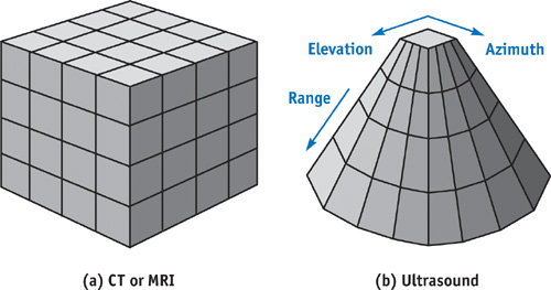
Figure 40-1 Sampling Grids for CT, MRI, and Ultrasound Data

Say you want to get a 3D ultrasound scan of some part of your anatomy. In the clinic, a sonographer first places an ultrasonic transducer on your skin. A transducer is basically an antenna, sensitive to sound waves operating at about 1 MHz or higher. It sends out inaudible sound pulses to the body and listens to the echoes, just like radar. Just like radar, ultrasound volumes are typically acquired in a grid that diverges as you move away from the transducer into the body. To give you an idea of the nature of ultrasound images, Figure 40-2 shows a 2D ultrasound image of a fetus. You can imagine the 3D version of the ultrasound volume: a truncated pyramid or a cone, similar to Figure 40-1b.

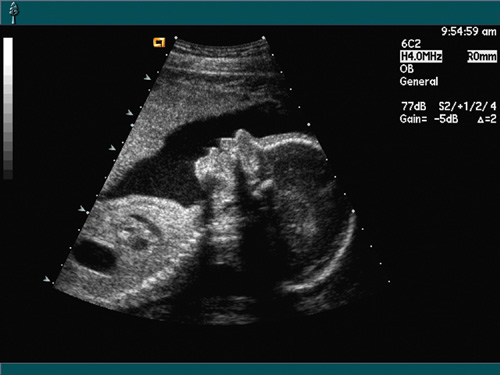
Figure 40-2 A 2D Ultrasound Image of a Fetal Head

Three-dimensional ultrasound data is acquired by an ultrasound scanner and stored in its local memory as a 3D array. The fastest-moving index of this 3D array corresponds to the distance away from the transducer, called the range direction (see Figure 40-1b). The next-fastest-moving index corresponds to the azimuth direction of the transducer. The slowest-moving index corresponds to the elevation direction of the transducer.

Ultrasound data can also be 4D, acquired in three spatial directions and in the time direction. You may have seen 4D ultrasound images of a fetal face acquired at an OB clinic. The number of volumes per second required for an application such as imaging a fetal face is far less than the number of volumes per second required for an application such as imaging the human heart. This is because the heart is moving rapidly and we need to acquire and volume render several 3D volumes per cardiac cycle to adequately visualize the heart motion.

Luckily, programmable vertex and fragment processors in modern GPUs, such as NVIDIA's GeForce FX and Quadro FX, have recently provided the means to volume render 4D ultrasound data acquired in non-Cartesian grids at the rates required for visualizing the human heart. A number of techniques exist to volume render 4D ultrasonic data. In this chapter, we walk through one such technique.

40.2 Introduction

Three-dimensional grid data sets, such as CT, MRI, and ultrasound data, can be volume rendered using texture mapping. A variety of techniques exists. See Chapter 39, "Volume Rendering Techniques," in this book and Hadwiger et al. 2002 for good reviews. In this chapter, we are using 3D textures. We first review how volume rendering is done using data such as CT and MRI in Cartesian grids. The sample OpenGL program VolumeRenderCartesian.cpp (which is on the book's CD and Web site) demonstrates how volume rendering is done using Cartesian grids. We do not go into great detail about this program here, but let's go through some basics.

40.2.1 Volume Rendering Data in a Cartesian Grid

Figure 40-3 shows the gist of volume rendering Cartesian data using 3D textures. The data is first loaded into the video memory as a 3D texture, using glTexImage3D. Then with alpha blending enabled, a series of cut-planes, all orthogonal to the viewing direction, is texture-mapped, starting from the cut-plane farthest from the viewer and proceeding to the cut-plane closest to the viewer. Remember, the cut-planes are all parallel to the computer screen. Let's call the coordinate system associated with the computer screen the cut-plane space. The data set can be rotated with respect to the computer screen. Let's call the coordinate system associated with the data set the data set space.

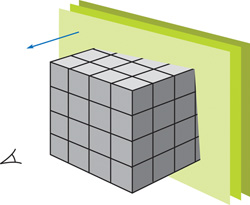
Figure 40-3 Volume Rendering 3D Cartesian Data

The content of a pixel in the frame buffer after the ith cut-plane is rendered, P_i , can be expressed as:

Equation 1

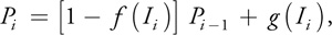
where P_i _- ₁ is the pixel content after the (i - 1)th cut-plane is rendered, I_i is the incoming fragment from the ith cut-plane, f() is an opacity function, and g() is an opacity-weighted transfer function. Both f() and g() are assumed to be in the range [0, 1]. Intuitively, this means that if the incoming fragment is opaque, the contributions from the fragments behind it are suppressed. Equation 1 can be implemented in OpenGL using alpha blending, with the blending function being GL_ONE_MINUS_SRC_ALPHA. The opacity-weighted transfer function produces the RGB values for the pixel, and the opacity function produces the alpha values of the pixel.

When texture-mapping the cut-planes, they can be specified using two different approaches: enclosing rectangles and polygons of intersections.

Enclosing Rectangles

The use of enclosing rectangles is the most straightforward way of texture-mapping cut-planes. The sample program VolumeRenderCartesian.cpp uses this technique. In this method, a series of quads enclosing the extent of the data set is drawn from back to front. You can store the coordinates of the vertices of the quads in the video memory for quick access for fast rendering. The only point to remember is to enable one of two ways to suppress texture mapping of the data outside the original data volume (that is, when any of the texture coordinates (s, t, r) is less than 0.0 or greater than 1.0). One can do this in one of three ways: (a) using clipping planes, (b) using GL_CLAMP_TO_BORDER_ARB for wrapping the texture coordinates and setting the border color to black, or (c) using GL_CLAMP_TO_EDGE for wrapping the texture coordinates and making the data values equal to 0 at the borders, as follows:

Data = 0 if s = 0.0, t = 0.0, r = 0.0, s = 1.0, t = 1.0 or r = 1.0.

Polygons of Intersection

This method is a bit more complex and requires you to find the polygon of intersection between a given cut-plane and the cube of data. You can ask either the CPU or the GPU (using a vertex program) to find it for you. Once you find the vertices of the polygon of intersection, you can then texture-map that polygon. This approach is faster than the other approach from the fragment program's point of view, because you are visiting only those fragments that are inside the cube of data. However, from the rasterizer's point of view, it is more demanding, because more triangles now need to be rasterized. Furthermore, each time the viewer changes the viewing direction with respect to the data set space, the program needs to recompute the polygons. If you are using the CPU to recompute the polygons, then you also need to upload the vertices of the polygons to the GPU before they are rendered, which can be time-consuming.

The sample program VolumeRenderCartesian.cpp uses the enclosing rectangles with clipping planes to render the cut-planes. Figure 40-4 shows a volume rendered image of a CT data set produced by the VolumeRenderCartesian.cpp program. You can rotate, zoom, and step through the volume when running this program. Type the key "h" when you have the keyboard focus on the graphics window to see help. The data set used for this visualization is 256x256x256 voxels.

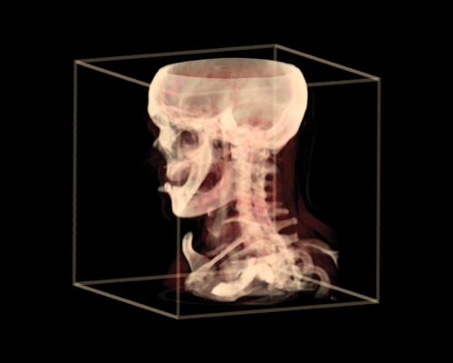
Figure 40-4 A Volume Rendered CT Data Set Acquired in a Cartesian Coordinate System

40.2.2 Volume Rendering Data in Pyramidal Grids

Now let's examine volume rendering of data acquired in pyramidal grids. There are several grids that have the property of diverging as you go into the body, including pyramidal, conical, spherical, and cylindrical grids. For simplicity, we use a pyramidal grid in this chapter because it lends itself to the kind of linear processing that GPUs are good at, as we see later. Furthermore, other types of grids, such as those shown in Figure 40-1b and Figure 40-2, can also be transformed into pyramidal grids by resampling the ultrasound data along the range direction, without loss of generality.

For explanation's sake, let's first look at two 2D cases: (a) Cartesian and (b) pyramidal grids, as shown in Figure 40-5. For each 2D grid, we acquire an ultrasound data sample at each of the grid points, forming a 2D data array. In general, ultrasound images have a lot more grid points. But here we are looking at only a 5x5 grid. In the Cartesian grid shown in Figure 40-5a, the vertical lines corresponding to constant s are called ultrasound lines. The transducer is located at the r = 0.0 plane. The ultrasound scanner fires each ultrasound line sequentially from left to right and samples data at each grid point to collect a 2D image. The texture coordinates (s, r) correspond to the azimuth and range directions of the transducer.

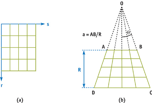
Figure 40-5 Cartesian and Pyramidal Grids in 2D

In the pyramidal grid shown in Figure 40-5b, the ultrasound lines all meet at a common point, O, called the apex. The extent of the transducer, AB, is called the aperture size. In this chapter, we use the concept of the normalized aperture size: a = AB/R, where R is the height of the pyramid (0 R 1.0). The angle AOB is called the apex angle, 2q. We can think of the pyramidal grid as being equivalent to the Cartesian grid, with the change that the s coordinate is scaled as a function of the r coordinate, linearly. We can easily accomplish this by using projective texture mapping, as we discuss later.

Figure 40-6 shows the 3D pyramidal grid. In order to generate the correct texture coordinates for the 3D pyramidal grid, we scale the s and t texture coordinates as a linear function of r, similar to the 2D pyramidal grid. The following are the steps of this algorithm:

Assuming that we are using a Cartesian grid, generate the texture coordinates inside the vertex program by mimicking OpenGL's automatic texture-coordinate-generation function, glTexGen.
The goal is to scale the s and t coordinates, but not the r coordinate, as a linear function of r. To do this, compute the following new texture coordinates inside the vertex program:
Equation 2

Equation 3

Equation 4

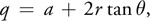
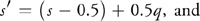
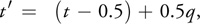
where s', t' and q are the new coordinates.
Then in a fragment program, do the scaling and texture lookup in a single step using the projective 3D texture lookup instruction. Keep in mind that you need to prevent the scaling performed on the r coordinate; otherwise, you get scaling along the r direction as well, generating a pyramidal data volume that appears to stretch more and more along the r direction as you go into the body. To avoid this, simply premultiply the r coordinate with the scale in the fragment program:
Equation 5

where r' is also a new texture coordinate. (Because this step is a nonlinear operation, we cannot do it in the vertex program, because the GPU then interpolates incorrect values for r' across each fragment.)
When all is said and done, the projective texture lookup instruction uses the following effective texture coordinates for texture lookup:
Equation 6

Equation 7

Equation 8

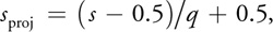
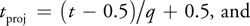
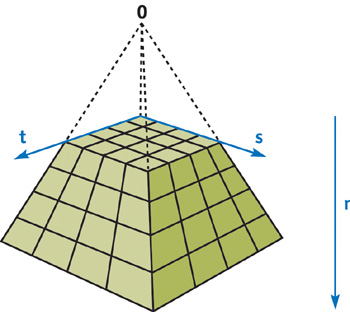
Figure 40-6 3D Pyramidal Grid

The cut-planes are specified as a series of enclosing rectangles as discussed earlier. The size of these rectangles is chosen such that they completely enclose the pyramidal grid. The sample OpenGL program, VolumeRenderPyramid.cpp, the vertex program, VolumeRenderPyramidV.cg, and the fragment program, VolumeRenderPyramidF.cg, illustrate our algorithm using the same CT data set used before in VolumeRenderCartesian.cpp. There is also an assembly version of the fragment program in VolumeRenderPyramidF.ocg. Now let's investigate the vertex and fragment programs.

The Vertex Program

We now go through our vertex program one line at a time, as shown in Listing 40-1 The input to this vertex program is the variable Position, containing the vertex coordinates. Ten uniform variables—ZoomFactor, Pyramid, ClipPlane0-5, ModelView, and ModelViewProj—are also input to this program. ZoomFactor contains the scale value used for zooming. Pyramid contains two parameters describing the geometry of the pyramidal grid: Pyramid.x, the normalized aperture size of the transducer, a, and Pyramid.y, two times the tangent of half of the apex angle, 2 tan . ClipPlane0 through ClipPlane5 contain the equations of the six clipping planes. ModelView and ModelViewProj contain the modelview matrix in the data set space and the modelview matrix concatenated with the projection matrix of the cut-plane space, respectively.

Example 40-1. `VolumeRenderPyramidV.cg`

 void VertexProgram(in float4  Position  : POSITION,                    out float4 hPosition : POSITION,                    out float4 hTex0     : TEX0,                    out float  hClip0    : CLP0,                    out float  hClip1    : CLP1,                    out float  hClip2    : CLP2,                    out float  hClip3    : CLP3,                    out float  hClip4    : CLP4,                    out float  hClip5    : CLP5,                    uniform float4 ZoomFactor,                    uniform float4 Pyramid,                    uniform float4 ClipPlane0,                    uniform float4 ClipPlane1,                    uniform float4 ClipPlane2,                    uniform float4 ClipPlane3,                    uniform float4 ClipPlane4,                    uniform float4 ClipPlane5,                    uniform float4x4 ModelView,                    uniform float4x4 ModelViewProj) {   // Compute the clip-space position   hPosition = mul(ModelViewProj, Position); 
  // Remove the zoom factor from the position coordinates   Position = Position * ZoomFactor; 
  // Compute the texture coordinates using the Cartesian grid   hTex0 = mul(ModelView, Position); 
  // Save original texture coordinates     float4 hTex0_Orig = hTex0 - float4(0.5, 0.5, 0.0, 0.0); 
  // Compute the scale for the texture coordinates in the     // pyramidal grid   hTex0.w = Pyramid.x + hTex0.z * Pyramid.y; 
  // Adjust for the texture coordinate offsets   hTex0.x = hTex0.x - 0.5 + 0.5 * hTex0.w;   hTex0.y = hTex0.y - 0.5 + 0.5 * hTex0.w;   // Clip pyramidal volume   hClip0 = dot(hTex0_Orig, ClipPlane0);   hClip1 = dot(hTex0_Orig, ClipPlane1);   hClip2 = dot(hTex0_Orig, ClipPlane2);   hClip3 = dot(hTex0_Orig, ClipPlane3);   hClip4 = dot(hTex0_Orig, ClipPlane4);   hClip5 = dot(hTex0_Orig, ClipPlane5); }

The outputs of this vertex program are the clip-space position of the vertex, hPosition; the texture coordinates, hTex0; and the clip distances, CLP0 through CLP5.

In the first line, we are computing the clip-space position of the vertex, and in the second line, we remove any scaling applied by the OpenGL program to the position coordinates. In the third line, we are computing the texture coordinates for the Cartesian coordinate system, mimicking OpenGL's glTexGen function. In line 4, we are saving the original content of the texture coordinates, shifted by 0.5 only in s and t directions, in hTex0_Orig for later use. And then comes the fun part. In line 5, we are computing the amount of stretching or scaling we have to do to the s and t texture coordinates for a given r coordinate. In lines 6 and 7, we are offsetting the origin of the s and t texture coordinates so that the scaling of s and t texture coordinates in the fragment program is performed around the central axis of the pyramid. Lines 8–13 compute the clipping values for the six planes bounding the pyramidal volume. Fragments containing clipping values less than zero are not drawn to the frame buffer.

The Fragment Program

The fragment program in Listing 40-2 takes it from where the vertex program left off. The input, inTex, is a variable containing the texture coordinates. There are two uniform inputs as well: USTexture and ColorMap. USTexture contains the 3D texture describing the 3D ultrasound volume. ColorMap is a color map table containing the opacity-weighted transfer and opacity functions. The output, sColor0, contains the fragment color.

In the first line, we are premultiplying the r coordinate with the scale. In the second line, we are looking up the texture value with the 3D ultrasound volume using projective texture mapping. In the third line, we are doing a 1D color map lookup to generate the colors to render according to the ultrasound data value.

Example 40-2. `VolumeRenderPyramidF.cg`

 void FragmentProgram(in float4 inTex : TEXCOORD0,                      out float4 sColor0 : COLOR0,                      const uniform sampler3D USTexture,                      const uniform sampler1D ColorMap) {   // Premultiply 'r' coordinate with the scale   inTex.z = inTex.z * inTex.w; 
  // Projective 3D texture lookup     float val = tex3Dproj(USTexture, inTex); 
  // Color map lookup   sColor0 = tex1D(ColorMap, val); }

Typically, the volume rendering speed is limited by the complexity of the fragment program (that is, it's fill-rate bound). Therefore, sometimes it is better to hand-tweak the fragment assembly code to get the maximum throughput, as shown in Listing 40-3.

Example 40-3. `VolumeRenderPyramidF.ocg`

 !!FP1.0 # NV_fragment_program generated by NVIDIA Cg compiler # cgc version 1.1.0003, build date Mar  4 2003  12:32:10 # command line args: -q -profile fp30 -entry FragmentProgram #vendor NVIDIA Corporation #version 1.0.02 #profile fp30 #program FragmentProgram #semantic FragmentProgram.USTexture #semantic FragmentProgram.ColorMap #var float4 inTex : $vin.TEXCOORD0 : TEXCOORD0 : 0 : 1 #var float4 sColor0 : $vout.COLOR0 : COLOR0 : 1 : 1 #var sampler3D USTexture :  : texunit 0 : 2 : 1 #var sampler1D ColorMap :  : texunit 1 : 3 : 1 MOVX H0, f[TEX0]; MULX H0.z, H0.z, H0.w; TXP  R0, H0, TEX0, 3D; TEX  o[COLR], R0.x, TEX1, 1D; END # 4 instructions, 1 R-regs, 1 H-regs. # End of program

In the first line, the incoming texture coordinate is loaded into one of the 12-bit fixed-point registers, H0. In the next line, the r component of the texture coordinate is premultiplied using the scale. Using 12-bit fixed-point math, we can accelerate the rendering speed significantly. In the third line, we are looking up the fragment value using 3D projective texture lookup. In the last line, we are looking up the color value of the fragment using a 1D color map lookup. And that's it!

Figure 40-7 shows a volume rendered image produced by the sample OpenGL program, VolumeRenderPyramid.cpp, which lets you play with the aperture size (keys "a"/"A") and the apex angle (keys "b"/"B") and see the effect on the screen. Press the "h" key to see Help.

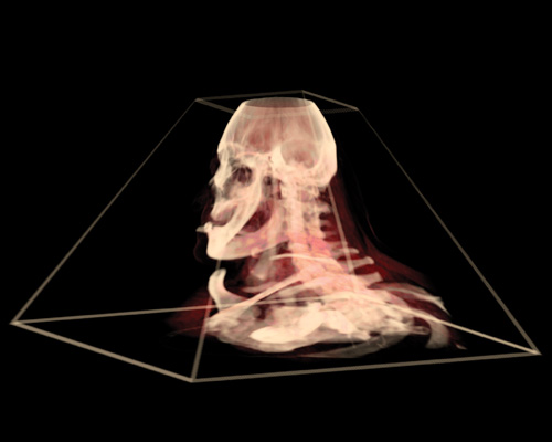
Figure 40-7 The CT Data Set Volume Rendered in a Pyramidal Coordinate System

Volume Rendering Ultrasound Data

The sample program VolumeRenderPyramidUS.cpp demonstrates the use of ultrasound data for volume rendering. The ultrasound data of a fetus in utero, acquired using an ACUSON Sequoia 512 ultrasound system, consists of 256x256x32 voxels. Note that in this case, due to the special geometry of the ultrasound probe used to acquire the data, we do not need to change the t coordinate as we did in Equation 7. We only need to scale the s coordinate as a linear function. This produces a pyramidal geometry consisting of a wedge-shaped volume.

40.3 Results

Figure 40-8 shows a volume rendered image of the face of a fetus using the projective texture mapping technique outlined in this chapter. The sample program VolumeRenderPyramidUS.cpp produces this image using 181 cut-planes. In the movie clip VolumeRenderPyramidUS.avi, if you look closely, you can see the fetus putting its tongue out and scratching its head.

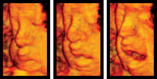
Figure 40-8 The Volume Rendered Image of a Fetal Face Using Projective Texture Mapping

40.4 Conclusion

GPUs have advanced to the point where it is possible to do volume rendering at the rapid rates required for 3D ultrasonic imaging. We have described how to do this for pyramidal grids using projective texture mapping. Using this as the framework, one can include a shading model and also reduce moiré artifacts by using techniques such as preintegrated volume rendering (Engel et al. 2001), with some frame-rate loss.

Note that Equations 6 and 7 can be implemented in a fragment program directly, without using projective texture mapping. This approach is slower compared to the approach we have taken in this chapter. This is because typical volume rendering applications are fill-rate bound, and implementing Equations 6 and 7 would require you to invert the value of r, which requires additional statements and hence runs more slowly.

Note also that we could have supplied a transfer function to the fragment program instead of an opacity-weighted transfer function, and generated the opacity-weighted color inside the fragment program by multiplying the opacity value with the color, sColor0. This would reduce the quantization artifacts at the expense of the frame rate, because it would require an additional statement.

40.5 References

Engel, Klaus, Martin Kraus, and Thomas Ertl. 2001. "High-Quality Pre-Integrated Volume Rendering Using Hardware-Accelerated Pixel Shading." Proceedings of the SIGGRAPH/Eurographics Workshop on Graphics Hardware 2001. Available online at http://wwwvis.informatik.uni-stuttgart.de/~engel/pre-integrated/paper_GraphicsHardware2001.pdf

Hadwiger, Markus, Joe Kniss, Klaus Engel, and Christof Rezk-Salama. 2002. "High-Quality Volume Graphics on Consumer PC Hardware." Course Notes 42, SIGGRAPH 2002. Available online at http://www.cs.utah.edu/~jmk/sigg_crs_02/course_42/course_42_notes_small.pdf

Copyright

Many of the designations used by manufacturers and sellers to distinguish their products are claimed as trademarks. Where those designations appear in this book, and Addison-Wesley was aware of a trademark claim, the designations have been printed with initial capital letters or in all capitals.

The authors and publisher have taken care in the preparation of this book, but make no expressed or implied warranty of any kind and assume no responsibility for errors or omissions. No liability is assumed for incidental or consequential damages in connection with or arising out of the use of the information or programs contained herein.

The publisher offers discounts on this book when ordered in quantity for bulk purchases and special sales. For more information, please contact:

U.S. Corporate and Government Sales
(800) 382-3419
corpsales@pearsontechgroup.com

For sales outside of the U.S., please contact:

International Sales
international@pearsoned.com

Visit Addison-Wesley on the Web: www.awprofessional.com

Library of Congress Control Number: 2004100582

GeForce™ and NVIDIA Quadro^® are trademarks or registered trademarks of NVIDIA Corporation.
RenderMan^® is a registered trademark of Pixar Animation Studios.
"Shadow Map Antialiasing" © 2003 NVIDIA Corporation and Pixar Animation Studios.
"Cinematic Lighting" © 2003 Pixar Animation Studios.
Dawn images © 2002 NVIDIA Corporation. Vulcan images © 2003 NVIDIA Corporation.

All rights reserved. No part of this publication may be reproduced, stored in a retrieval system, or transmitted, in any form, or by any means, electronic, mechanical, photocopying, recording, or otherwise, without the prior consent of the publisher. Printed in the United States of America. Published simultaneously in Canada.

For information on obtaining permission for use of material from this work, please submit a written request to:

Pearson Education, Inc.
Rights and Contracts Department
One Lake Street
Upper Saddle River, NJ 07458

Text printed on recycled and acid-free paper.

5 6 7 8 9 10 QWT 09 08 07

5th Printing September 2007