GPU Gems

GPU Gems is now available, right here, online. You can purchase a beautifully printed version of this book, and others in the series, at a 30% discount courtesy of InformIT and Addison-Wesley.

The CD content, including demos and content, is available on the web and for download.

Chapter 8. Simulating Diffraction

Jos Stam
Alias Systems

8.1 What Is Diffraction?

Most surface reflection models in computer graphics ignore the wavelike effects of natural light. This is fine whenever the surface detail is much larger than the wavelength of light (roughly a micron). For surfaces with small-scale detail such as a compact disc, however, wave effects cannot be neglected. The small-scale surface detail causes the reflected waves to interfere with one another. This phenomenon is known as diffraction.

Diffraction causes the reflected light from these surfaces to exhibit many colorful patterns, as you can see in the subtle reflections from a compact disc. Other surfaces that exhibit diffraction are now common and are mass-produced to create funky wrapping paper, colorful toys, and fancy watermarks, for example.

In this chapter we show how to model diffraction effects on arbitrary surfaces in real time. This is possible thanks to the programmable hardware available on current graphics cards. In particular, we provide a complete implementation of our shader using the Cg programming language. Our shader is a simplified version of the more general model described in our SIGGRAPH 1999 paper (Stam 1999).

8.1.1 The Wave Theory of Light

At a fundamental level, light behaves as a wave. In fact, the ray theory of light used in computer graphics is an approximation of this wave theory. Waves appear in many physical theories of natural phenomena. This is not surprising, because Nature abounds with repeating patterns, both in space and in time.

The simple, one-dimensional wave in Figure 8-1 is completely described by its wavelength and amplitude A. The wavelength characterizes the oscillating pattern, while the amplitude determines the intensity of the wave. Visible light comprises a superposition of these waves, with wavelengths ranging from 0.5 microns (ultraviolet) to 1 micron (infrared). The color of a light source is determined by the distribution of amplitudes of the waves emanating from it. For example, a reddish light source is composed mainly of waves whose wavelengths peak in the 1-micron range, but sunlight has an equal distribution of waves across all wavelengths.

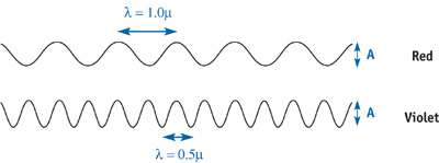
Figure 8-1 Light Waves Range from Ultraviolet to Infrared

8.1.2 The Physics of Diffraction

Our simple diffraction shader models the reflection of light from a surface commonly known as a diffraction grating. A diffraction grating is composed of a set of parallel, narrow reflecting bands separated by a distance d . Figure 8-2a shows a cross section of this surface.

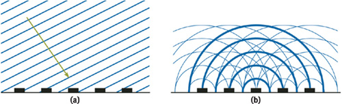
Figure 8-2 A Diffraction Grating

A light wave emanating from a light source is usually approximated by a planar wave. A cross section of this wave is depicted by drawing the lines that correspond to the crests of the wave. Unlike a simple, one-dimensional wave, a planar wave requires a specified direction, in addition to its wavelength and amplitude. Figure 8-2a depicts a planar wave incident on our diffraction grating. Note that the spacing between the lines corresponds to the wavelength . When this type of planar wave hits the diffraction grating, it generates a spherical wave at each band, as shown in Figure 8-2b. The wavelength of the spherical waves is the same as that of the incoming planar, and their crests are depicted similarly. The only difference is that the crests lie on concentric circles instead of parallel lines. The reflected wave at any receiving point away from the surface is equal to the sum of the spherical waves at that location.

The main difference between the wave theory and the usual ray theory is that the amplitudes do not simply add up. Waves interfere. We illustrate this phenomenon in Figure 8-3, where we show two extreme cases. In the first case (a), the two waves are "in phase" and the amplitudes add up, as in the ray theory. In the second case (b), the waves cancel each other, resulting in a wave of zero amplitude. These two cases illustrate that waves can interfere both positively and negatively. In general, the resulting wave lies somewhere in between these two extremes. The first case is, however, the one we are most interested in: When waves interfere in phase, they produce the maximum possible intensity, which eventually will be observed at the receiver.

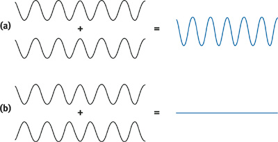
Figure 8-3 Wave Interference

We now explain in more detail the notion of waves being in phase. As is usual in this situation, we assume that the light source and the receiver are "far away" from the surface, as compared to the size of the surface detail. This is reasonable because the surface detail is a couple of microns wide, and we often observe a surface from a distance of 1 meter. That's six orders of magnitude in scale. In this case, we can assume that all the waves emanating from the surface and ending up at the receiver are parallel. Therefore, the waves reaching the receiver are exactly in phase when the paths from the light source to the receiver for different bands differ only by multiples of the wavelength . Let ₁ be the angle of the direction of the incident planar wave and ₂ be the angle to the receiver.

Then, from Figure 8-4 and using some basic trigonometry, we conclude that the waves are in phase whenever:

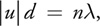
where n is an arbitrary positive integer and u = sin ₁ - sin ₂. This relation gives us exactly the wavelengths that interfere to give a maximum intensity at the receiver. These wavelengths are:

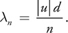
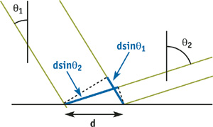
Figure 8-4 Angles Used for Computing the Difference in Phase Between Reflected Waves

Because n is arbitrary, this gives us an infinite number of wavelengths. However, only the wavelengths in the range [0.5, 1] microns correspond to visible light. So this gives us a range of possible values for n in terms of |u| and the spacing d:

Consequently, the color of the light at the receiver is equal to the sum of the colors of all waves having wavelengths given by the preceding formula.

What is the color corresponding to a given wavelength? As stated previously, the colors range from red to violet in a rainbow fashion. Although the exact color can be determined theoretically for a specific wavelength, we rely on a simple approximation instead. All that we require is a rainbow map, with colors ranging from violet to red, mimicking the rainbow. Let C() = (R(), G(), B()) be such a map, returning an RGB value for each wavelength in the interval [0.5, 1] microns. Then the color of the light reaching the observer is given by summing the colors C(|u|d/n) for each valid n. Notice that when u = 0 (exact reflection), all wavelengths contribute to the reflection. We will deal with this case separately in the implementation of our shader.

8.2 Implementation

We now describe our implementation of the theory as a vertex program in Cg. Of course, we could have implemented it using a fragment program. Our implementation should work for any mesh, as long as a "tangent vector" is provided, plus the normal and position for each vertex. The tangent vectors supply the local direction of the narrow bands on the surface. For a compact disc, they are in the direction of the tracks, as shown in Figure 8-5.

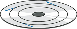
Figure 8-5 Tangent Vectors for the Compact Disc

The complete implementation of our vertex program is given in Listing 8-1.

Example 8-1. The Diffraction Shader Vertex Program

 float3 blend3 (float3 x)  {    float3 y = 1 - x * x;    y = max(y, float3 (0, 0, 0));    return (y);  } 
 void vp_Diffraction (    in float4 position : POSITION,    in float3 normal   : NORMAL,    in float3 tangent  : TEXCOORD0,    out float4 positionO : POSITION,    out float4 colorO    : COLOR,    uniform float4x4 ModelViewProjectionMatrix,    uniform float4x4 ModelViewMatrix,    uniform float4x4 ModelViewMatrixIT,    uniform float r,    uniform float d,    uniform float4 hiliteColor,    uniform float3 lightPosition,    uniform float3 eyePosition  )  {    float3 P = mul(ModelViewMatrix, position).xyz;    float3 L = normalize(lightPosition - P);    float3 V = normalize(eyePosition - P);    float3 H = L + V;    float3 N = mul((float3x3)ModelViewMatrixIT, normal);    float3 T = mul((float3x3)ModelViewMatrixIT, tangent);    float u = dot(T, H) * d;    float w = dot(N, H);    float e = r * u / w;    float c = exp(-e * e);    float4 anis = hiliteColor * float4(c.x, c.y, c.z, 1); 
   if (u < 0) u = -u; 
   float4 cdiff = float4(0, 0, 0, 1);    for (int n = 1; n < 8; n++)    {      float y = 2 * u / n - 1;      cdiff.xyz += blend3(float3(4 * (y - 0.75), 4 * (y - 0.5),                                 4 * (y - 0.25)));    } 
   positionO = mul(ModelViewProjectionMatrix, position); 
   colorO = cdiff + anis; }

The code computes the colorful diffraction pattern and the main anisotropic highlight corresponding to the u = 0 case.

Let's first describe the computation of the diffraction pattern. From the halfway vector between the light source and the receiver (not normalized), we compute the u value by projecting it onto the local tangent vector. From this value and the spacing d, we then compute the wavelengths that interfere in phase. If we compute the wavelength correctly, we should first determine the range of n values that are valid, and then sum over the corresponding colors. However, currently the Cg compiler unrolls its for loops; therefore the size of the loop is limited by the allowable size of the vertex program. So we decided to use a fixed number of allowable n's in our implementation. The value we currently use is 8. In later versions of our shader, we might want to allow variable for loops, depending on |u| and d, as explained in Section 8.1.2.

To determine the color corresponding to a given wavelength, we use a simple approximation of a rainbow map. Basically, the map should range from violet to red and produce most colors in the rainbow. We found that a simple blend of three identical bump functions (which peak in the blue, green, and red regions) worked well, as shown in Figure 8-6.

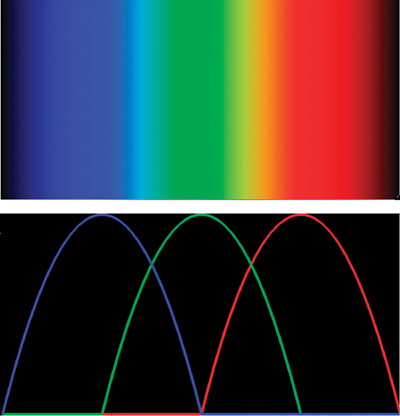
Figure 8-6 The Rainbow Color Map Used in the Shader

More precisely, our bump function is equal to:

Then, using this function, we can define the RGB components of our rainbow map as:

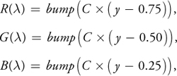
where y = 2 - 1 maps the wavelength to the [0, 1] micron range, and C is a shape parameter that controls the appearance of the rainbow map. In our implementation we found that C = 4.0 gave acceptable results. This is just one possible rainbow map. In fact, a better solution might be to use a one-dimensional texture map or a table lookup.

The case when u = 0 is dealt with using a simple anisotropic shader. Theoretically, this should just correspond to an infinitely thin white highlight. However, the irregularities in the bumps on each of the bands of the diffraction grating (on a compact disc, for example) cause a visible spread of the highlight. Therefore, we decided to model this contribution with a simple anisotropic shader by Greg Ward (Ward 1992). The spread of the highlight is modeled using a roughness parameter r and its color is given by the hiliteColor parameter. The resulting expression for this contribution is:

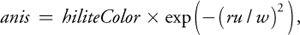
where w is the component of the halfway vector in the normal direction.

The final color is simply the sum of the colorful diffraction pattern and the anisotropic highlight.

8.3 Results

We wrote a program that uses the diffraction vertex shader to visualize the reflection from a compact disc. The compact disc is modeled as a set of thin quads. Of course, our shader is not restricted to the geometry of a compact disc: all that is required is that a tangent direction be provided for each vertex.

In addition, we added a thin transparent layer on the compact disc with a Fresnel-like reflection shader. This layer reflects the environment more strongly for glancing angles. Figure 8-7 shows three snapshots of our real-time demo, with the CD in three different positions. Figure 8-8 shows our diffraction shader applied to a surface where we have texture-mapped the principal direction of anisotropy.

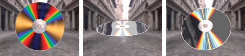
Figure 8-7 Three Snapshots of Our Compact Disc Real-Time Demo

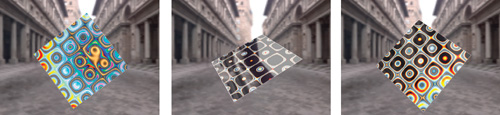
Figure 8-8 Three Snapshots of a Surface with a Texture-Mapped Principal Direction of Anisotropy

8.4 Conclusion

We have shown how to implement a simple diffraction shader that demonstrates some of the wavelike features of natural light. Derivations for more complicated surface detail can be found in our SIGGRAPH 1999 paper (Stam 1999). Readers who are interested in learning more about the wave theory of light can consult the classic book Principles of Optics (Born and Wolf 1999), which we have found useful. Possible directions of future work might include more complicated surfaces than a simple diffraction grating. For example, it would be challenging to model the reflection from metallic paints, which consist of several scattering layers. The small pigments in these paints cause many visible wavelike effects. Developing such a model would have many applications in the manufacturing of new paints.

8.5 References

Born, Max, and Emil Wolf. 1999. Principles of Optics: Electromagnetic Theory of Propagation, Interference and Diffraction to Light, 7th ed. Cambridge University Press.

Stam, Jos, 1999. "Diffraction Shaders." In Proceedings of SIGGRAPH 99, pp. 101–110.

Ward, Greg. 1992. "Measuring and Modeling Anisotropic Reflection." In Proceedings of SIGGRAPH 92, pp. 265–272.

Copyright

Many of the designations used by manufacturers and sellers to distinguish their products are claimed as trademarks. Where those designations appear in this book, and Addison-Wesley was aware of a trademark claim, the designations have been printed with initial capital letters or in all capitals.

The authors and publisher have taken care in the preparation of this book, but make no expressed or implied warranty of any kind and assume no responsibility for errors or omissions. No liability is assumed for incidental or consequential damages in connection with or arising out of the use of the information or programs contained herein.

The publisher offers discounts on this book when ordered in quantity for bulk purchases and special sales. For more information, please contact:

U.S. Corporate and Government Sales
(800) 382-3419
corpsales@pearsontechgroup.com

For sales outside of the U.S., please contact:

International Sales
international@pearsoned.com

Visit Addison-Wesley on the Web: www.awprofessional.com

Library of Congress Control Number: 2004100582

GeForce™ and NVIDIA Quadro^® are trademarks or registered trademarks of NVIDIA Corporation.
RenderMan^® is a registered trademark of Pixar Animation Studios.
"Shadow Map Antialiasing" © 2003 NVIDIA Corporation and Pixar Animation Studios.
"Cinematic Lighting" © 2003 Pixar Animation Studios.
Dawn images © 2002 NVIDIA Corporation. Vulcan images © 2003 NVIDIA Corporation.

All rights reserved. No part of this publication may be reproduced, stored in a retrieval system, or transmitted, in any form, or by any means, electronic, mechanical, photocopying, recording, or otherwise, without the prior consent of the publisher. Printed in the United States of America. Published simultaneously in Canada.

For information on obtaining permission for use of material from this work, please submit a written request to:

Pearson Education, Inc.
Rights and Contracts Department
One Lake Street
Upper Saddle River, NJ 07458

Text printed on recycled and acid-free paper.

5 6 7 8 9 10 QWT 09 08 07

5th Printing September 2007

Part II: Lighting and Shadows

Part III: Materials

Part IV: Image Processing

Part V: Performance and Practicalities

Part VI: Beyond Triangles

Preface