GPU Gems
GPU Gems is now available, right here, online. You can purchase a beautifully printed version of this book, and others in the series, at a 30% discount courtesy of InformIT and Addison-Wesley.
The CD content, including demos and content, is available on the web and for download.
Chapter 26. The OpenEXR Image File Format
Florian Kainz
Industrial Light & Magic
Rod Bogart
Industrial Light & Magic
Drew Hess
Industrial Light & Magic
Most images created on a GPU are fleeting and exist for only a fraction of a second. But occasionally you create one worth keeping. When you do, it's best to store it in an image file format that retains the high dynamic range possible in the NVIDIA half type and stores additional data channels, as well.
In this chapter, we describe the OpenEXR image file format, give examples of reading and writing GPU image buffers, and discuss issues associated with image display.
26.1 What Is OpenEXR?
OpenEXR is a high-dynamic-range image file format developed by Industrial Light & Magic (ILM) for use in computer imaging applications. The OpenEXR Web site, www.openexr.org, has full details on the image file format itself. This section summarizes some of the key features for storing high-dynamic-range images.
26.1.1 High-Dynamic-Range Images
Display devices for digital images, such as computer monitors and video projectors, usually have a dynamic range of about 500 to 1. This means the brightest pixel in an image is never more than 500 times brighter than the darkest pixel.
Most image file formats are designed to match a typical display's dynamic range: values stored in the pixels go from 0.0, representing "black," to 1.0, representing the display's maximum intensity, or "white." To keep image files small, pixel values are usually encoded as eight- or ten-bit integers (0–255 or 0–1023, respectively), which is just enough to match the display's accuracy.
As long as we only want to present images on a display, file formats with a dynamic range of 0 to 1 are adequate. There is no point in storing pixels that are brighter than the monitor's white, or in storing pixels with more accuracy than what the display can reproduce.
However, if we intend to process an image, or if we want to use an image as an environment map for 3D rendering, then it is desirable to have more information in the image file. Pixels should be stored with more accuracy than the typical eight or ten bits, and the range of possible pixel values should be essentially unlimited. File formats that allow storing pixel values outside the 0-to-1 range are called high-dynamic-range (HDR) formats. By performing image processing on HDR data and quantizing to fewer bits only for display, the best-quality image can be shown.
Here is a simple example that demonstrates why having a high dynamic range is desirable for image processing (other applications for HDR images are presented in Section 26.6).
Figure 26-1 shows a photograph of a scene with a rather high dynamic range. In the original scene, the flame of the oil lamp on the left was about 100,000 times brighter than the shadow under the small dish in the center.
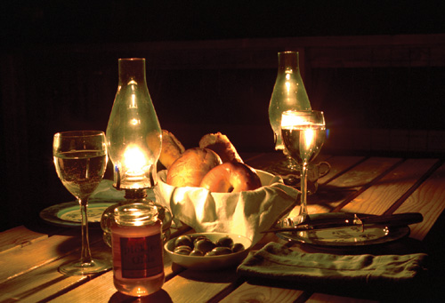
Figure 26-1 A Scene with a High Dynamic Range
The way the image was exposed caused some areas to be brighter than 1.0. On a computer monitor, those areas are clipped and displayed as white or as unnaturally saturated orange hues.
We might attempt to correct the white and orange areas by making the image darker. However, if the original image has been stored in a low-dynamic-range file format, for example, JPEG, darkening produces a rather ugly image. The areas around the flames become gray, as in Figure 26-2.
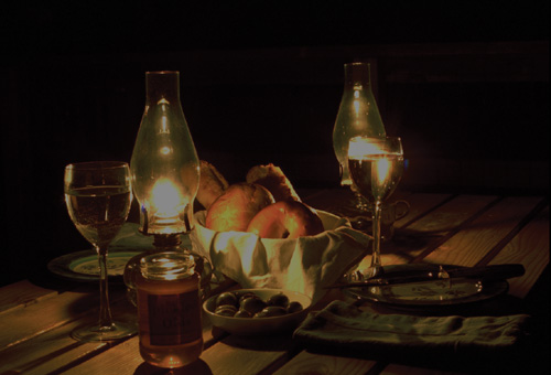
Figure 26-2 Darker Version of
If the original image has been stored in an HDR file format such as OpenEXR, which preserves bright pixel values rather than clipping them at 1.0, then darkening produces an image that still looks natural. See Figure 26-3.
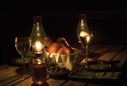
Figure 26-3 High-Dynamic-Range Version of , Made Darker
26.1.2 A "Half" Format
Early in 2003, ILM released a new HDR file format with 16-bit floating-point color-component values. Because the IEEE 754 floating-point specification does not define a 16-bit format, ILM created a half format that matches NVIDIA's 16-bit format. The half type provides an excellent storage structure for high-dynamic-range image content. This type is directly supported in the OpenEXR format.
The 16-bit, or "half-precision," floating-point format is modeled after the IEEE 754 single-precision and double-precision formats. A half-precision number consists of a sign bit, a 5-bit exponent, and a 10-bit mantissa. The smallest and largest possible exponent values are reserved for representing zero, denormalized numbers, infinities, and NaNs.
In OpenEXR's C++ implementation, numbers of type half generally behave like the built-in C++ floating-point types, float and double. The half, float, and double types can be mixed freely in arithmetic expressions. Here are a few examples:
half a(3.5);
float b(a + sqrt(a));
a += b;
b += a;
b = a + 7;
26.1.3 Range of Representable Values
The most obvious benefit of half is the range of values that can be represented with only 16 bits. We can store a maximum image value of 65504.0 and a minimum value of 5.96–8. This is a dynamic range of a trillion to one. Any image requiring this range would be extremely rare, but images with a million-to-one range do occur, and thus they are comfortably represented with a half.
Photographers measure dynamic range in stops, where a single stop is a factor of 2. In an image with five stops of range, the brightest region is 32 times brighter than the darkest region. A range of one-million to one is 20 stops in photographic terms.
26.1.4 Color Resolution
The second, less obvious benefit of half is the color resolution. Each stop contains 1024 distinct values. This makes OpenEXR excellent for normal-dynamic-range images as well. In an eight-stop image that ranges from 1.0 down to 0.0039 (or 2–8), the half format will provide 8192 values per channel, whereas an 8-bit, gamma 2.2 image will have only 235 values (21 through 255).
26.1.5 C++ Interface
To make writing and reading OpenEXR files easy, ILM designed the file format together with a C++ programming interface. OpenEXR provides three levels of access to the image files: (1) a general interface for writing and reading files with arbitrary sets of image channels; (2) a specialized interface for RGBA (red, green, blue, and alpha channels, or some subset of those); and (3) a C-callable version of the programming interface that supports reading and writing OpenEXR files from programs written in C.
The examples in this chapter use the RGBA C++ interface.
26.2 The OpenEXR File Structure
An OpenEXR file consists of two main parts: the header and the pixels.
26.2.1 The Header
The header is a list of attributes that describe the pixels. An attribute is a named data item of an arbitrary type. In order for OpenEXR files written by one program to be read by other programs, certain required attributes must be present in all OpenEXR file headers. These attributes are presented in Table 26-1.
Table 26-1. Required Attributes in OpenEXR Headers
|
Name |
Description |
|
displayWindow |
The image's resolution [1] |
|
dataWindow |
Crop and offset |
|
pixelAspectRatio |
Width divided by the height of a pixel when the image is displayed with the correct aspect ratio |
|
channels |
Description of the image channels stored in the file |
|
compression |
The compression method applied to the pixel data of all channels in the file |
|
lineOrder |
The order in which the scan lines are stored in the file (increasing y or decreasing y) |
|
screenWindowWidth, screenWindowCenter |
The perspective projection that produced the image |
In addition to the required attributes, a program can include optional attributes in the file's header. Often it is necessary to annotate images with additional data that's appropriate for a particular application, such as computational history, color profile information, or camera position and view direction. These data can be packaged as extra attributes in the image file's header.
26.2.2 The Pixels
The pixels of an image are stored as separate channels. With the general library interface, you can write RGBA and as many additional channels as necessary. Each channel can have a different data type, so the RGBA data can be half (16 bits), while a z-depth channel can be written as float (32 bits).
26.3 OpenEXR Data Compression
OpenEXR offers three different data compression methods, each of which has differing trade-offs in speed versus compression ratio. All three compression schemes, as listed in Table 26-2, are lossless; compressing and uncompressing does not alter the pixel data.
Table 26-2. OpenEXR Supported Compression Options
|
Name |
Description |
|
PIZ |
A wavelet transform is applied to the pixel data, and the result is Huffman-encoded. This scheme tends to provide the best compression ratio for photographic images. Files are compressed and decompressed at about the same speed. For photographic images with film grain, the files are reduced to between 35 and 55 percent of their uncompressed size. |
|
ZIP |
Differences between horizontally adjacent pixels are compressed using the open-source zlib library. ZIP decompression is faster than PIZ decompression, but ZIP compression is significantly slower. Compressed photographic images are often 45 to 55 percent of their uncompressed size. |
|
RLE |
Run-length encoding of differences between horizontally adjacent pixels. This method is fast, and it works well for images with large flat areas. However, for photographic images, the compressed file size is usually 60 to 75 percent of the uncompressed size. |
Optionally, the pixels can be stored in uncompressed form. If stored on a fast file system, uncompressed files can be written and read significantly faster than compressed files.
26.4 Using OpenEXR
The electronic materials accompanying this book contain the full source code for a simple image-playback program, along with the associated Cg shader code.
This section provides excerpts of the code to demonstrate reading an OpenEXR image file, displaying the image buffer with OpenGL, performing a simple compositing operation, and writing the result to an OpenEXR file.
26.4.1 Reading and Displaying an OpenEXR Image
The simple code in Listing 26-1 reads an OpenEXR file into an internal image buffer. Note that the OpenEXR library makes use of exceptions, so errors such as "file not found" are handled in a catch block. There is no need to explicitly close the file because it is closed by the C++ destructor for the RgbaInputFile object.
Example 26-1. Reading an OpenEXR Image File
Imf::Rgba *pixelBuffer;
try
{
  Imf::RgbaInputFile in(fileName);
  Imath::Box2i win = in.dataWindow();
  Imath::V2i dim(win.max.x - win.min.x + 1, win.max.y - win.min.y + 1);
  pixelBuffer = new Imf::Rgba[dim.x * dim.y];
  int dx = win.min.x;
  int dy = win.min.y;
  in.setFrameBuffer(pixelBuffer - dx - dy * dim.x, 1, dim.x);
  in.readPixels(win.min.y, win.max.y);
}
catch (Iex::BaseExc &e)
{
  std::cerr < < e.what() < < std::endl;
  //
  // Handle exception.
  //
}
Once the buffer is filled, the code segment in Listing 26-2 binds the image to a texture for display with a Cg fragment shader (see Section 26.5 for more details). The full program invokes this display code to play back multiple frames.
Example 26-2. Binding an Image to a Texture
GLenum target = GL_TEXTURE_RECTANGLE_NV;
glGenTextures(2, imageTexture);
glBindTexture(target, imageTexture);
glTexParameteri(target, GL_TEXTURE_MIN_FILTER, GL_NEAREST);
glTexParameteri(target, GL_TEXTURE_MAG_FILTER, GL_NEAREST);
glTexParameteri(target, GL_TEXTURE_WRAP_S, GL_CLAMP_TO_EDGE);
glTexParameteri(target, GL_TEXTURE_WRAP_T, GL_CLAMP_TO_EDGE);
glPixelStorei(GL_UNPACK_ALIGNMENT, 1);
glTexImage2D(target, 0, GL_FLOAT_RGBA16_NV, dim.x, dim.y, 0, GL_RGBA,
             GL_HALF_FLOAT_NV, pixelBuffer);
glActiveTextureARB(GL_TEXTURE0_ARB);
glBindTexture(target, imageTexture);
glBegin(GL_QUADS);
glTexCoord2f(0.0, 0.0);
glVertex2f(0.0, 0.0);
glTexCoord2f(dim.x, 0.0);
glVertex2f(dim.x, 0.0);
glTexCoord2f(dim.x, dim.y);
glVertex2f(dim.x, dim.y);
glTexCoord2f(0.0, dim.y);
glVertex2f(0.0, dim.y);
glEnd();
26.4.2 Rendering and Writing an OpenEXR Image
Images rendered by the GPU can be saved in OpenEXR files. Often, we want to create a foreground image and a background image and combine them later. The example in Listing 26-3 uses a pbuffer to do a simple compositing operation, and then it writes the result to an OpenEXR file. In the code fragment, we read the two input images (which are already open) into the allocated image buffers, and then we call a compositing routine and write the result.
Example 26-3. Compositing Two Images and Writing an OpenEXR File
//
// Read A and B.
//
Imath::V2i dim(dataWinA.max.x - dataWinA.min.x + 1,
               dataWinA.max.y - dataWinA.min.y + 1);
int dx = dataWinA.min.x;
int dy = dataWinA.min.y;
Imf::Array<Imf::Rgba> imgA(dim.x *dim.y);
Imf::Array<Imf::Rgba> imgB(dim.x *dim.y);
inA.setFrameBuffer(imgA - dx - dy * dim.x, 1, dim.x);
inA.readPixels(dataWinA.min.y, dataWinA.max.y);
inB.setFrameBuffer(imgB - dx - dy * dim.x, 1, dim.x);
inB.readPixels(dataWinB.min.y, dataWinB.max.y);
//
// Do the comp, overwrite image B with the result.
//
Comp::over(dim, imgA, imgB, imgB);
//
// Write comp'ed image.
Imf::RgbaOutputFile outC(outputFilename.c_str(), dpyWinA, dataWinA,
                         Imf::WRITE_RGBA);
outC.setFrameBuffer(imgB - dx - dy * dim.x, 1, dim.x);
outC.writePixels(dim.y);
The call to Comp::over is implemented simply as a call to the routine shown in Listing 26-4 (Comp::comp) with the name of a Cg shader that performs an over operation. Full details of over and various other compositing operators are found in Porter and Duff 1984. The GlFloatPbuffer class (which is provided in the accompanying materials) hides the mechanics of creating and deleting a floating-point pbuffer. Note that we can get half data from the pbuffer with glReadPixels without loss of precision and without clamping.
Listings 26-5 through 26-7 are the Cg shaders for the over operation and for in and out operations, respectively.
Example 26-4. Compositing into a Pbuffer
void Comp::comp(const Imath::V2i &dim, const Imf::Rgba *imageA,
                const Imf::Rgba *imageB, Imf::Rgba *imageC,
                const char *cgProgramName)
{
  GlFloatPbuffer pbuffer(dim);
  pbuffer.activate();
  //
  // Set up default ortho view.
  //
  glLoadIdentity();
  glViewport(0, 0, dim.x, dim.y);
  glOrtho(0, dim.x, dim.y, 0, -1, 1);
  //
  // Create input textures.
  //
  GLuint inTex[2];
  glGenTextures(2, inTex);
  GLenum target = GL_TEXTURE_RECTANGLE_NV;
  glActiveTextureARB(GL_TEXTURE0_ARB);
  glBindTexture(target, inTex[0]);
  glTexParameteri(target, GL_TEXTURE_MIN_FILTER, GL_NEAREST);
  glTexParameteri(target, GL_TEXTURE_MAG_FILTER, GL_NEAREST);
  glTexParameteri(target, GL_TEXTURE_WRAP_S, GL_CLAMP_TO_EDGE);
  glTexParameteri(target, GL_TEXTURE_WRAP_T, GL_CLAMP_TO_EDGE);
  glPixelStorei(GL_UNPACK_ALIGNMENT, 1);
  glTexImage2D(target, 0, GL_FLOAT_RGBA16_NV, dim.x, dim.y, 0, GL_RGBA,
               GL_HALF_FLOAT_NV, imageA);
  glActiveTextureARB(GL_TEXTURE1_ARB);
  glBindTexture(target, inTex[1]);
  glTexParameteri(target, GL_TEXTURE_MIN_FILTER, GL_NEAREST);
  glTexParameteri(target, GL_TEXTURE_MAG_FILTER, GL_NEAREST);
  glTexParameteri(target, GL_TEXTURE_WRAP_S, GL_CLAMP_TO_EDGE);
  glTexParameteri(target, GL_TEXTURE_WRAP_T, GL_CLAMP_TO_EDGE);
  glPixelStorei(GL_UNPACK_ALIGNMENT, 1);
  glTexImage2D(target, 0, GL_FLOAT_RGBA16_NV, dim.x, dim.y, 0, GL_RGBA,
               GL_HALF_FLOAT_NV, imageB);
  //
  // Compile the Cg program and load it.
  //
  cgSetErrorCallback(cgErrorCallback);
  CGcontext cgcontext = cgCreateContext();
  CGprogram cgprog = cgCreateProgramFromFile(
      cgcontext, CG_SOURCE, cgProgramName, CG_PROFILE_FP30, 0, 0);
  cgGLLoadProgram(cgprog);
  cgGLBindProgram(cgprog);
  cgGLEnableProfile(CG_PROFILE_FP30);
  //
  // Render to pbuffer.
  //
  glEnable(GL_FRAGMENT_PROGRAM_NV);
  glBegin(GL_QUADS);
  glTexCoord2f(0.0, 0.0);
  glVertex2f(0.0, 0.0);
  glTexCoord2f(dim.x, 0.0);
  glVertex2f(dim.x, 0.0);
  glTexCoord2f(dim.x, dim.y);
  glVertex2f(dim.x, dim.y);
  glTexCoord2f(0.0, dim.y);
  glVertex2f(0.0, dim.y);
  glEnd();
  glDisable(GL_FRAGMENT_PROGRAM_NV);
  //
  // Read pixels out of pbuffer.
  //
  glReadPixels(0, 0, dim.x, dim.y, GL_RGBA, GL_HALF_FLOAT_NV, imageC);
  checkGlErrors();
  pbuffer.deactivate();
}
Example 26-5. Cg Shader for an "Over" Operation
void over(float2 wpos
          : WPOS, out half4 c
          : COLOR, uniform float2 dim, uniform samplerRECT A,
            uniform samplerRECT B)
{
  half4 a = texRECT(A, wpos.xy);
  half4 b = texRECT(B, wpos.xy);
  c = a + (1 - a.a) * b;
}
Example 26-6. Cg Shader for an "In" Operation
void in(float2 wpos
        : WPOS, out half4 c
        : COLOR, uniform float2 dim, uniform samplerRECT A,
          uniform samplerRECT B)
{
  half4 a = texRECT(A, wpos.xy);
  half4 b = texRECT(B, wpos.xy);
  c = b.a * a;
}
Example 26-7. Cg Shader for an "Out" Operation
void out(float2 wpos
         : WPOS, out half4 c
         : COLOR, uniform float2 dim, uniform samplerRECT A,
           uniform samplerRECT B)
{
  half4 a = texRECT(A, wpos.xy);
  half4 b = texRECT(B, wpos.xy);
  c = (1 - b.a) * a;
}
26.5 Linear Pixel Values
We prefer to store linear images in OpenEXR files. The word linear has different meanings to different people—for us, an image is in linear color space if the values in the image are proportional to the relative scene luminances represented. When we double the number, we double the light. To make a scene half as bright—that is, make it a stop darker—we divide each image value by two. As we'll describe later, this has implications for how images should be displayed.
Most image-processing algorithms assume linear images. The standard compositing operation over performs a linear blend of the foreground and the background based on an alpha channel. When the alpha is truly a coverage mask, it indicates the percentage of light that should leak through from the background. This works correctly when the images represent linear amounts of light. In addition to image processing, antialiasing is best done in linear space (Blinn 2002).
Software rendering is usually performed in linear space as well. With higher-quality rendering available in the GPU, it is correct to do the hardware rendering in linear space. When the image is viewed, it must be gamma-corrected. Although gamma also has many meanings in the graphics community, we are referring here to correcting for the monitor gamma. Monitors used for image display have circuits that cause the monitor's light output to have a power-law relationship to the frame buffer value. Because we assume that OpenEXR images are linear, we tell the display program the gamma of the monitor so the program can apply the inverse gamma to the image for display.
A typical monitor has a gamma of 2.2. You can measure this with a light meter (preferably a high-quality one). If you don't have a light meter, see the method described in Berger 2003. When you display a white value of 1.0, the meter may display a value such as 92 nit (1 nit equals 1 candela per square meter). For a second data point, we display a gray patch. (We don't use a black patch because a black region will have suspect light readings; also, we're about to do some log math, which is undefined at zero.)
Let's assume the 0.5 gray value gives a luminance of 20 nit. Remember, this value of 0.5 is the digital value in the frame buffer, with no other processing downstream before the digital-to-analog converters. The monitor's output luminance, L(v), as a function of the input value, v, is:
L(v) = Lm · v,
where v is in the range from 0.0 to 1.0 and Lm is the monitor's maximum output luminance. From this we can derive gamma () as:
To apply gamma correction to the linear image data, we simply raise the image value to the power of 1 over the monitor gamma. We demonstrate this in the simple fragment shader in Listing 26-8.
Example 26-8. Gamma-Correcting an Image for Display
struct Out
{
  half4 color : COLOR;
};
Out main(float2 texCoord
         : TEXCOORD0, uniform samplerRECT image, uniform float gamma)
{
  half4 pixel = h4texRECT(image, texCoord);
  Out output;
  output.color = pow(pixel, gamma);
  return output;
}
The playback program lets the user change the exposure of the image. The image is linear before gamma correction, so we just multiply by a constant and pass the result to the power function. See Listing 26-9.
Example 26-9. Adjusting an Image's Exposure
Out main(float2 texCoord
         : TEXCOORD0, uniform samplerRECT image, uniform float gamma,
           uniform float expMult)
{
  half4 pixel = h4texRECT(image, texCoord);
  pixel.rgb *= expMult;
  Out output;
  output.color = pow(pixel, gamma);
  return output;
}
Finally, the image may need some overall color correction to look right. The reasons for this may be aesthetic, or it may be that the image is intended to look as if it were shown on a different display device. For example, if you want your image on the monitor to look like film, you can perform a simulation of the film behavior just before gamma correction. Often, digital image designers have to use lighting tricks to achieve the right look. Instead, we prefer to do our lighting and rendering in linear space and simulate the behavior of film at display time. In the basic example shown in Listing 26-10, we provide a three-channel lookup table that contains a simple S-shaped film simulation curve.
This shader uses a trick to do the lookup function. The samplerRECT types that are used as lookup tables store a half for each possible input half. The simplest encoding of this is a sampler rect with dimensions 1x66536. Because of limitations in current GPUs, this rect is too large. So instead, we fold the lookup table into a 256x256 texture, which we index using the pack_2half and unpack_4ubyte Cg Standard Library functions. These take the given half input value and split it into two indices for the 256x256 lookups.
Example 26-10. Using a Lookup Table to Simulate the Look of Photographic Film
half lookup(samplerRECT lut, half h)
{
  float f = pack_2half(h.xx);
  half4 bytes = unpack_4ubyte(f);
  return h1texRECT(lut, bytes.xy * 256.0);
}
Out main(float2 texCoord
         : TEXCOORD0, uniform samplerRECT image, uniform samplerRECT lutR,
           uniform samplerRECT lutG, uniform samplerRECT lutB,
           uniform float gamma, uniform float expMult)
{
  half4 c = h4texRECT(image, texCoord) * expMult;
  c.r = lookup(lutR, c.r);
  c.g = lookup(lutG, c.g);
  c.b = lookup(lutB, c.b);
  Out output;
  output.color = pow(c, gamma);
  return output;
}
Fully commented versions of these routines are provided, along with the OpenGL code for binding the various textures and displaying the image, on the book's CD and Web site.
26.6 Creating and Using HDR Images
HDR images can be created synthetically on the GPU or in software. They can also be captured from the real world. High-dynamic-range cameras do exist. For example, Spheron's SpheroCam captures 26-stop dynamic-range panoramas. With a regular camera, you can take multiple exposures and construct a single HDR image using software such as Greg Ward's PhotoSphere or Paul Debevec's HDRShop.
Lighting can be done in 3D scenes with a global illumination model using high-dynamic-range images rather than individual light sources. In Debevec 1998, synthetic objects are rendered with Radiance software. In Ng et al. 2003, realistic rendering of diffuse surfaces, including shadows, is done in real time on NVIDIA hardware. Both methods use environment maps instead of light sources; the maps must have a wide enough dynamic range to represent the brightest regions in the environment (for example, the Sun) without clipping.
Image processing also benefits from a wider dynamic range. For example, depth-of-field blurring spreads individual pixels over large areas. When an individual pixel is very bright, spreading it out should result in many reasonably bright pixels. But if a bright pixel, for example a specular highlight, has been clamped to zero-to-one before blurring, the blurred highlight is unnaturally dim. A similar effect can be seen with motion blur. Even performing a simple color correction can require high-dynamic-range data, as seen in Section 26.1.1.
In Figure 26-4a, we have a high-dynamic-range image of an automobile engine. The highlights range much higher than 1.0. For Figure 26-4b, we first converted the image to a low-dynamic-range file format, which clamped the pixels to zero-to-one. Then we applied a depth-of-field blur. In Figure 26-4c, we blurred the full range of data read from the OpenEXR file.
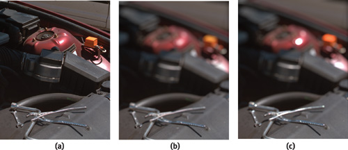
Figure 26-4 Blurring an Image with Very Bright Highlights
In previous sections, we assumed that values above 1.0 are clamped when an HDR image is displayed. This can work reasonably well, and in fact, it was the method used for printing the figures in this chapter. However, it is often possible to do better. Several effective techniques for reducing the dynamic range without significantly altering the subjective appearance of the image, known as tone mapping, have been published in recent years—for example, Fattal et al. 2002 and Durand and Dorsey 2002. Alternatively, future displays may show HDR imagery directly. For example, Seetzen et al. 2003 describes a prototype HDR display with a dynamic range of 120,000 to 1.
26.7 Conclusion
OpenEXR was originally released for GNU/Linux and Irix, and through the efforts of the open-source community, it was ported to Mac OS X and Windows. The OpenEXR library has been proven in the visual effects production environment of Industrial Light & Magic.
In addition to NVIDIA, a growing number of vendors support the OpenEXR format in their software applications. For more information, visit the OpenEXR Web site at www.openexr.org.
26.8 References
Berger, Robert W. 2003. "Why Do Images Appear Darker on Some Displays?" Article on Web site. http://www.bberger.net/rwb/gamma.html
Blinn, Jim. 2002. Jim Blinn's Corner: Notation, Notation, Notation, pp. 133–146. Morgan Kaufmann.
Debevec, Paul. 1998. "Rendering Synthetic Objects into Real Scenes." In Computer Graphics (Proceedings of SIGGRAPH 98), pp. 189–198.
Durand, Frédo, and Julie Dorsey. 2002. "Fast Bilateral Filtering for the Display of High-Dynamic-Range Images." In Computer Graphics (Proceedings of SIGGRAPH 2002), pp. 257–266.
Fattal, Raanan, Dani Lischinski, and Michael Werman. 2002. "Gradient Domain High Dynamic Range Compression." In Computer Graphics (Proceedings of SIGGRAPH 2002), pp. 249–256.
Ng, Ren, Ravi Ramamoorthi, and Pat Hanrahan. 2003. "All-Frequency Shadows Using Non-linear Wavelet Lighting Approximation." In Computer Graphics (Proceedings of SIGGRAPH 2003), pp. 376–381.
Porter, Thomas, and Tom Duff. 1984. "Compositing Digital Images." In Computer Graphics 18(3) (Proceedings of SIGGRAPH 84), pp. 253–259.
Seetzen, H., W. Stürzlinger, A. Vorozcovs, H. Wilson, I. Ashdown, G. Ward, and L. Whitehead. 2003. "High Dynamic Range Display System." Emerging technologies demonstration at SIGGRAPH 2003.
Copyright
Many of the designations used by manufacturers and sellers to distinguish their products are claimed as trademarks. Where those designations appear in this book, and Addison-Wesley was aware of a trademark claim, the designations have been printed with initial capital letters or in all capitals.
The authors and publisher have taken care in the preparation of this book, but make no expressed or implied warranty of any kind and assume no responsibility for errors or omissions. No liability is assumed for incidental or consequential damages in connection with or arising out of the use of the information or programs contained herein.
The publisher offers discounts on this book when ordered in quantity for bulk purchases and special sales. For more information, please contact:
U.S. Corporate and Government Sales
(800) 382-3419
corpsales@pearsontechgroup.com
For sales outside of the U.S., please contact:
International Sales
international@pearsoned.com
Visit Addison-Wesley on the Web: www.awprofessional.com
Library of Congress Control Number: 2004100582
GeForce™ and NVIDIA Quadro® are trademarks or registered trademarks of NVIDIA Corporation.
RenderMan® is a registered trademark of Pixar Animation Studios.
"Shadow Map Antialiasing" © 2003 NVIDIA Corporation and Pixar Animation Studios.
"Cinematic Lighting" © 2003 Pixar Animation Studios.
Dawn images © 2002 NVIDIA Corporation. Vulcan images © 2003 NVIDIA Corporation.
Copyright © 2004 by NVIDIA Corporation.
All rights reserved. No part of this publication may be reproduced, stored in a retrieval system, or transmitted, in any form, or by any means, electronic, mechanical, photocopying, recording, or otherwise, without the prior consent of the publisher. Printed in the United States of America. Published simultaneously in Canada.
For information on obtaining permission for use of material from this work, please submit a written request to:
Pearson Education, Inc.
Rights and Contracts Department
One Lake Street
Upper Saddle River, NJ 07458
Text printed on recycled and acid-free paper.
5 6 7 8 9 10 QWT 09 08 07
5th Printing September 2007
- Contributors
- Copyright
- Foreword
- Part I: Natural Effects
-
- Chapter 1. Effective Water Simulation from Physical Models
- Chapter 2. Rendering Water Caustics
- Chapter 3. Skin in the "Dawn" Demo
- Chapter 4. Animation in the "Dawn" Demo
- Chapter 5. Implementing Improved Perlin Noise
- Chapter 6. Fire in the "Vulcan" Demo
- Chapter 7. Rendering Countless Blades of Waving Grass
- Chapter 8. Simulating Diffraction
- Part II: Lighting and Shadows
-
- Chapter 9. Efficient Shadow Volume Rendering
- Chapter 10. Cinematic Lighting
- Chapter 11. Shadow Map Antialiasing
- Chapter 12. Omnidirectional Shadow Mapping
- Chapter 13. Generating Soft Shadows Using Occlusion Interval Maps
- Chapter 14. Perspective Shadow Maps: Care and Feeding
- Chapter 15. Managing Visibility for Per-Pixel Lighting
- Part III: Materials
- Part IV: Image Processing
- Part V: Performance and Practicalities
-
- Chapter 28. Graphics Pipeline Performance
- Chapter 29. Efficient Occlusion Culling
- Chapter 30. The Design of FX Composer
- Chapter 31. Using FX Composer
- Chapter 32. An Introduction to Shader Interfaces
- Chapter 33. Converting Production RenderMan Shaders to Real-Time
- Chapter 34. Integrating Hardware Shading into Cinema 4D
- Chapter 35. Leveraging High-Quality Software Rendering Effects in Real-Time Applications
- Chapter 36. Integrating Shaders into Applications
- Part VI: Beyond Triangles
- Preface