GPU Gems
GPU Gems is now available, right here, online. You can purchase a beautifully printed version of this book, and others in the series, at a 30% discount courtesy of InformIT and Addison-Wesley.
The CD content, including demos and content, is available on the web and for download.
Chapter 38. Fast Fluid Dynamics Simulation on the GPU
Mark J. Harris
University of North Carolina at Chapel Hill
This chapter describes a method for fast, stable fluid simulation that runs entirely on the GPU. It introduces fluid dynamics and the associated mathematics, and it describes in detail the techniques to perform the simulation on the GPU. After reading this chapter, you should have a basic understanding of fluid dynamics and know how to simulate fluids using the GPU. The source code accompanying this book demonstrates the techniques described in this chapter.
38.1 Introduction
Fluids are everywhere: water passing between riverbanks, smoke curling from a glowing cigarette, steam rushing from a teapot, water vapor forming into clouds, and paint being mixed in a can. Underlying all of them is the flow of fluids. All are phenomena that we would like to portray realistically in interactive graphics applications. Figure 38-1 shows examples of fluids simulated using the source code provided with this book.
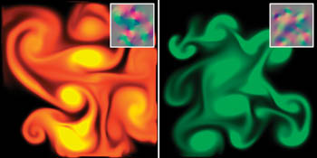
Figure 38-1 Colored "Dye" Carried by a Swirling Fluid
Fluid simulation is a useful building block that is the basis for simulating a variety of natural phenomena. Because of the large amount of parallelism in graphics hardware, the simulation we describe runs significantly faster on the GPU than on the CPU. Using an NVIDIA GeForce FX, we have achieved a speedup of up to six times over an equivalent CPU simulation.
38.1.1 Our Goal
Our goal is to assist you in learning a powerful tool, not just to teach you a new trick. Fluid dynamics is such a useful component of more complex simulations that treating it as a black box would be a mistake. Without understanding the basic physics and mathematics of fluids, using and extending the algorithms we present would be very difficult. For this reason, we did not skimp on the mathematics here. As a result, this chapter contains many potentially daunting equations. Wherever possible, we provide clear explanations and draw connections between the math and its implementation.
38.1.2 Our Assumptions
The reader is expected to have at least a college-level calculus background, including a basic grasp of differential equations. An understanding of vector calculus principles is helpful, but not required (we will review what we need). Also, experience with finite difference approximations of derivatives is useful. If you have ever implemented any sort of physical simulation, such as projectile motion or rigid body dynamics, many of the concepts we use will be familiar.
38.1.3 Our Approach
The techniques we describe are based on the "stable fluids" method of Stam 1999. However, while Stam's simulations used a CPU implementation, we choose to implement ours on graphics hardware because GPUs are well suited to the type of computations required by fluid simulation. The simulation we describe is performed on a grid of cells. Programmable GPUs are optimized for performing computations on pixels, which we can consider to be a grid of cells. GPUs achieve high performance through parallelism: they are capable of processing multiple vertices and pixels simultaneously. They are also optimized to perform multiple texture lookups per cycle. Because our simulation grids are stored in textures, this speed and parallelism is just what we need.
This chapter cannot teach you everything about fluid dynamics. The scope of the simulation concepts that we can cover here is necessarily limited. We restrict ourselves to simulation of a continuous volume of fluid on a two-dimensional rectangular domain. Also, we do not simulate free surface boundaries between fluids, such as the interface between sloshing water and air. There are many extensions to these basic techniques. We mention a few of these at the end of the chapter, and we provide pointers to further reading about them.
We use consistent mathematical notation throughout the chapter. In equations, italics are used for variables that represent scalar quantities, such as pressure, p. Boldface is used to represent vector quantities, such as velocity, u. All vectors in this chapter are assumed to be two-dimensional.
Section 38.2 provides a mathematical background, including a discussion of the equations that govern fluid flow and a review of basic vector calculus concepts and notation. It then discusses the approach to solving the equations. Section 38.3 describes implementation of the fluid simulation on the GPU. Section 38.4 describes some applications of the simulation, Section 38.5 presents extensions, and Section 38.6 concludes the chapter.
38.2 Mathematical Background
To simulate the behavior of a fluid, we must have a mathematical representation of the state of the fluid at any given time. The most important quantity to represent is the velocity of the fluid, because velocity determines how the fluid moves itself and the things that are in it. The fluid's velocity varies in both time and space, so we represent it as a vector field.
A vector field is a mapping of a vector-valued function onto a parameterized space, such as a Cartesian grid. (Other spatial parameterizations are possible, but for purposes of this chapter we assume a two-dimensional Cartesian grid.) The velocity vector field of our fluid is defined such that for every position x = (x, y), there is an associated velocity at time t, u(x, t) = (u(x, t), v(x, t), w(x, t)), as shown in Figure 38-2.
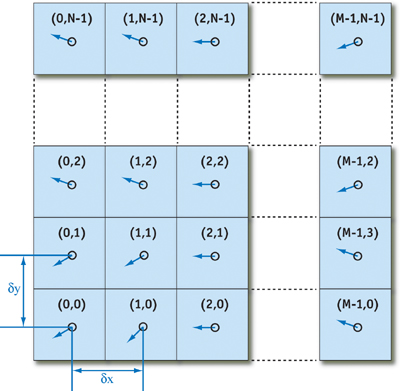
Figure 38-2 The Fluid Velocity Grid
The key to fluid simulation is to take steps in time and, at each time step, correctly determine the current velocity field. We can do this by solving a set of equations that describes the evolution of the velocity field over time, under a variety of forces. Once we have the velocity field, we can do interesting things with it, such as using it to move objects, smoke densities, and other quantities that can be displayed in our application.
38.2.1 The Navier-Stokes Equations for Incompressible Flow
In physics it's common to make simplifying assumptions when modeling complex phenomena. Fluid simulation is no exception. We assume an incompressible, homogeneous fluid.
A fluid is incompressible if the volume of any subregion of the fluid is constant over time. A fluid is homogeneous if its density, , is constant in space. The combination of incompressibility and homogeneity means that density is constant in both time and space. These assumptions are common in fluid dynamics, and they do not decrease the applicability of the resulting mathematics to the simulation of real fluids, such as water and air.
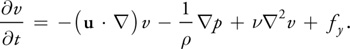
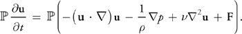
We simulate fluid dynamics on a regular Cartesian grid with spatial coordinates x = (x, y) and time variable t. The fluid is represented by its velocity field u(x, t), as described earlier, and a scalar pressure field p(x, t). These fields vary in both space and time. If the velocity and pressure are known for the initial time t = 0, then the state of the fluid over time can be described by the Navier-Stokes equations for incompressible flow:
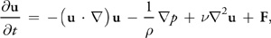
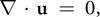
where is the (constant) fluid density, is the kinematic viscosity, and F = (fx , fy ) represents any external forces that act on the fluid. Notice that Equation 1 is actually two equations, because u is a vector quantity:

Thus, we have three unknowns (u, v, and p) and three equations.
The Navier-Stokes equations may initially seem daunting, but like many complex concepts, we can better understand them by breaking them into simple pieces. Don't worry if the individual mathematical operations in the equations don't make sense yet. First, we will try to understand the different factors influencing the fluid flow. The four terms on the right-hand side of Equation 1 are accelerations. We'll look at them each in turn.
38.2.2 Terms in the Navier-Stokes Equations
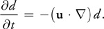
Advection
The velocity of a fluid causes the fluid to transport objects, densities, and other quantities along with the flow. Imagine squirting dye into a moving fluid. The dye is transported, or advected, along the fluid's velocity field. In fact, the velocity of a fluid carries itself along just as it carries the dye. The first term on the right-hand side of Equation 1 represents this self-advection of the velocity field and is called the advection term.
Pressure
Because the molecules of a fluid can move around each other, they tend to "squish" and "slosh." When force is applied to a fluid, it does not instantly propagate through the entire volume. Instead, the molecules close to the force push on those farther away, and pressure builds up. Because pressure is force per unit area, any pressure in the fluid naturally leads to acceleration. (Think of Newton's second law, F = m a.) The second term, called the pressure term, represents this acceleration.
Diffusion
From experience with real fluids, you know that some fluids are "thicker" than others. For example, molasses and maple syrup flow slowly, but rubbing alcohol flows quickly. We say that thick fluids have a high viscosity. Viscosity is a measure of how resistive a fluid is to flow. This resistance results in diffusion of the momentum (and therefore velocity), so we call the third term the diffusion term.
External Forces
The fourth term encapsulates acceleration due to external forces applied to the fluid. These forces may be either local forces or body forces. Local forces are applied to a specific region of the fluid—for example, the force of a fan blowing air. Body forces, such as the force of gravity, apply evenly to the entire fluid.
We will return to the Navier-Stokes equations after a quick review of vector calculus. For a detailed derivation and more details, we recommend Chorin and Marsden 1993 and Griebel et al. 1998.
38.2.3 A Brief Review of Vector Calculus
Equations 1 and 2 contain three different uses of the symbol
 (often pronounced "del"), which is also known as the nabla operator. The three applications of nabla
are the gradient, the divergence, and the Laplacian operators, as shown in Table 38-1. The subscripts i
and j used in the expressions in the table refer to discrete locations on a Cartesian grid, and
dx and y are the grid spacing in the x and y dimensions, respectively (see
Figure 38-2).
(often pronounced "del"), which is also known as the nabla operator. The three applications of nabla
are the gradient, the divergence, and the Laplacian operators, as shown in Table 38-1. The subscripts i
and j used in the expressions in the table refer to discrete locations on a Cartesian grid, and
dx and y are the grid spacing in the x and y dimensions, respectively (see
Figure 38-2).
Table 38-1. Vector Calculus Operators Used in Fluid Simulation
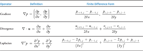
The gradient of a scalar field is a vector of partial derivatives of the scalar field. Divergence, which appears in Equation 2, has an important physical significance. It is the rate at which "density" exits a given region of space. In the Navier-Stokes equations, it is applied to the velocity of the flow, and it measures the net change in velocity across a surface surrounding a small piece of the fluid. Equation 2, the continuity equation, enforces the incompressibility assumption by ensuring that the fluid always has zero divergence. The dot product in the divergence operator results in a sum of partial derivatives (rather than a vector, as with the gradient operator). This means that the divergence operator can be applied only to a vector field, such as the velocity, u = (u, v).
Notice that the gradient of a scalar field is a vector field, and the divergence of a vector field is a scalar
field. If the divergence operator is applied to the result of the gradient operator, the result is the
Laplacian operator
·
=
2.
If the grid cells are square (that is, if dx = y, which we assume for the remainder of this
chapter), the Laplacian simplifies to:
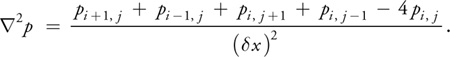
The Laplacian operator appears commonly in physics, most notably in the form of diffusion equations, such as
the heat equation. Equations of the form
2
x = b are known as Poisson equations. The case where b = 0 is
Laplace's equation, which is the origin of the Laplacian operator. In Equation 2, the Laplacian is
applied to a vector field. This is a notational simplification: the operator is applied separately to each
scalar component of the vector field.
38.2.4 Solving the Navier-Stokes Equations
The Navier-Stokes equations can be solved analytically for only a few simple physical configurations. However, it is possible to use numerical integration techniques to solve them incrementally. Because we are interested in watching the evolution of the flow over time, an incremental numerical solution suits our needs.
As with any algorithm, we must divide the solution of the Navier-Stokes equations into simple steps. The method we use is based on the stable fluids technique described in Stam 1999. In this section we describe the mathematics of each of these steps, and in Section 38.3 we describe their implementation using the Cg language on the GPU.
First we need to transform the equations into a form that is more amenable to numerical solution. Recall that the Navier-Stokes equations are three equations that we can solve for the quantities u, v, and p. However, it is not obvious how to solve them. The following section describes a transformation that leads to a straightforward algorithm.
The Helmholtz-Hodge Decomposition
Basic vector calculus tells us that any vector v can be decomposed into a set of basis vector
components whose sum is v. For example, we commonly represent vectors on a Cartesian grid as a
pair of distances along the grid axes: v = (x, y). The same vector can be
written v = x î + y
 ,
where î and
are unit basis vectors aligned to the axes of the grid.
,
where î and
are unit basis vectors aligned to the axes of the grid.
In the same way that we can decompose a vector into a sum of vectors, we can also decompose a vector field into
a sum of vector fields. Let D be the region in space, or in our case the plane, on which our fluid is
defined. Let this region have a smooth (that is, differentiable) boundary,
 D,
with normal direction n. We can use the following theorem, as stated in Chorin and Marsden
1993.
D,
with normal direction n. We can use the following theorem, as stated in Chorin and Marsden
1993.
Helmholtz-Hodge Decomposition Theorem
A vector field w on D can be uniquely decomposed in the form:
where u has zero divergence and is parallel to
We use the theorem without proof. For details and a proof of this theorem, refer to Section 1.3 of Chorin and Marsden 1993.
This theorem states that any vector field can be decomposed into the sum of two other vector fields: a divergence-free vector field, and the gradient of a scalar field. It also says that the divergence-free field goes to zero at the boundary. It is a powerful tool, leading us to two useful realizations.
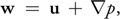
First Realization
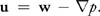
Solving the Navier-Stokes equations involves three computations to update the velocity at each time step: advection, diffusion, and force application. The result is a new velocity field, w, with nonzero divergence. But the continuity equation requires that we end each time step with a divergence-free velocity. Fortunately, the Helmholtz-Hodge Decomposition Theorem tells us that the divergence of the velocity can be corrected by subtracting the gradient of the resulting pressure field:
Second Realization
The theorem also leads to a method for computing the pressure field. If we apply the divergence operator to both sides of Equation 7, we obtain:

But since Equation 2 enforces that
·
u = 0, this simplifies to:
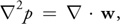
which is a Poisson equation (see Section 38.2.3) for the pressure of the fluid, sometimes called the Poisson-pressure equation. This means that after we arrive at our divergent velocity, w, we can solve Equation 10 for p, and then use w and p to compute the new divergence-free field, u, using Equation 8. We'll return to this later.
Now we need a way to compute w. To do this, let's return to our comparison of vectors and
vector fields. From the definition of the dot product, we know that we can find the projection of a vector
r onto a unit vector
 by computing the dot product of r and
.
The dot product is a projection operator for vectors that maps a vector r onto its component in
the direction of
.
We can use the Helmholtz-Hodge Decomposition Theorem to define a projection operator,
by computing the dot product of r and
.
The dot product is a projection operator for vectors that maps a vector r onto its component in
the direction of
.
We can use the Helmholtz-Hodge Decomposition Theorem to define a projection operator,
 , that
projects a vector field w onto its divergence-free component, u. If we apply
to Equation 7, we get:
, that
projects a vector field w onto its divergence-free component, u. If we apply
to Equation 7, we get:
)
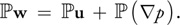
But by the definition of
,
w =
u = u. Therefore,
(p)
= 0. Now let's use these ideas to simplify the Navier-Stokes equations.
First, we apply our projection operator to both sides of Equation 1:
Because u is divergence-free, so is the derivative on the left-hand side, so
(
u/t)
=
u/t.
Also,
(p)
= 0, so the pressure term drops out. We're left with the following equation:
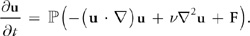
The great thing about this equation is that it symbolically encapsulates our entire algorithm for simulating fluid flow. We first compute what's inside the parentheses on the right-hand side. From left to right, we compute the advection, diffusion, and force terms. Application of these three steps results in a divergent velocity field, w, to which we apply our projection operator to get a new divergence-free field, u. To do so, we solve Equation 10 for p, and then subtract the gradient of p from w, as in Equation 8.
In a typical implementation, the various components are not computed and added together, as in Equation 11.
Instead, the solution is found via composition of transformations on the state; in other words, each component
is a step that takes a field as input, and produces a new field as output. We can define an operator
 that is equivalent to the solution of Equation 11 over a single time step. The operator is defined as the
composition of operators for advection (
that is equivalent to the solution of Equation 11 over a single time step. The operator is defined as the
composition of operators for advection (
 ), diffusion (
 ), force application (
 ), and projection (
):
), and projection (
):

Thus, a step of the simulation algorithm can be expressed
 The operators are applied right to left; first advection, followed by diffusion, force application, and
projection. Note that time is omitted here for clarity, but in practice, the time step must be used in the
computation of each operator. Now let's look more closely at the advection and diffusion steps, and then
approach the solution of Poisson equations.
The operators are applied right to left; first advection, followed by diffusion, force application, and
projection. Note that time is omitted here for clarity, but in practice, the time step must be used in the
computation of each operator. Now let's look more closely at the advection and diffusion steps, and then
approach the solution of Poisson equations.
Advection
Advection is the process by which a fluid's velocity transports itself and other quantities in the fluid. To compute the advection of a quantity, we must update the quantity at each grid point. Because we are computing how a quantity moves along the velocity field, it helps to imagine that each grid cell is represented by a particle. A first attempt at computing the result of advection might be to update the grid as we would update a particle system. Just move the position, r, of each particle forward along the velocity field the distance it would travel in time t:
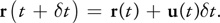
You might recognize this as Euler's method; it is a simple method for explicit (or forward) integration of ordinary differential equations. (There are more accurate methods, such as the midpoint method and the Runge-Kutta methods.)
There are two problems with this approach: The first is that simulations that use explicit methods for advection are unstable for large time steps, and they can "blow up" if the magnitude of u(t)t is greater than the size of a single grid cell. The second problem is specific to GPU implementation. We implement our simulation in fragment programs, which cannot change the locations of the fragments they are writing. This forward-integration method requires the ability to "move" the particles, so it cannot be implemented on current GPUs.
The solution is to invert the problem and use an implicit method (Stam 1999). Rather than advecting quantities by computing where a particle moves over the current time step, we trace the trajectory of the particle from each grid cell back in time to its former position, and we copy the quantities at that position to the starting grid cell. To update a quantity q (this could be velocity, density, temperature, or any quantity carried by the fluid), we use the following equation:

Not only can we easily implement this method on the GPU, but as Stam showed, it is stable for arbitrary time steps and velocities. Figure 38-3 depicts the advection computation at the cell marked with a double circle. Tracing the velocity field back in time leads to the green x. The four grid values nearest the green x (connected by a green square in the figure) are bilinearly interpolated, and the result is written to the starting grid cell.
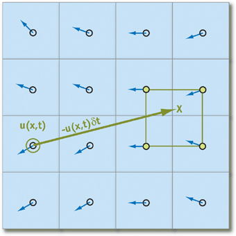
Figure 38-3 Computing Fluid Advection
Viscous Diffusion
As explained earlier, viscous fluids have a certain resistance to flow, which results in diffusion (or dissipation) of velocity. A partial differential equation for viscous diffusion is:
As in advection, we have a choice of how to solve this equation. An obvious approach is to formulate an explicit, discrete form in order to develop a simple algorithm:

In this equation,
2
is the discrete form of the Laplacian operator, Equation 3. Like the explicit Euler method for computing
advection, this method is unstable for large values of dt and v. We follow Stam's lead again
and use an implicit formulation of Equation 14:
where I is the identity matrix. This formulation is stable for arbitrary time steps and viscosities. This equation is a (somewhat disguised) Poisson equation for velocity. Remember that our use of the Helmholtz-Hodge decomposition results in a Poisson equation for pressure. These equations can be solved using an iterative relaxation technique.
Solution of Poisson Equations
We need to solve two Poisson equations: the Poisson-pressure equation and the viscous diffusion equation. Poisson equations are common in physics and well understood. We use an iterative solution technique that starts with an approximate solution and improves it every iteration.
The Poisson equation is a matrix equation of the form Ax = b, where
x is the vector of values for which we are solving (p or u in our
case), b is a vector of constants, and A is a matrix. In our case,
A is implicitly represented in the Laplacian operator
2,
so it need not be explicitly stored as a matrix. The iterative solution technique we use starts with an initial
"guess" for the solution, x (0), and each step k produces an improved
solution, x (k). The superscript notation indicates the iteration number.
The simplest iterative technique is called Jacobi iteration. A derivation of Jacobi iteration for general matrix
equations can be found in Golub and Van Loan 1996.
More sophisticated methods, such as conjugate gradient and multigrid methods, converge faster, but we use Jacobi iteration because of its simplicity and easy implementation. For details and examples of more sophisticated solvers, see Bolz et al. 2003, Goodnight et al. 2003, and Krüger and Westermann 2003.
Equations 10 and 15 appear different, but both can be discretized using Equation 3 and rewritten in the form:
where and are constants. The values of x, b, , and are
different for the two equations. In the Poisson-pressure equation, x represents p, b
represents
·
w, a = -(x)2, and = 4.
[1] For the viscous
diffusion equation, both x and b represent u, =
(x)2/t, and = 4 + .
We formulate the equations this way because it lets us use the same code to solve either equation. To solve the equations, we simply run a number of iterations in which we apply Equation 16 at every grid cell, using the results of the previous iteration as input to the next (x ( k +1) becomes x ( k )). Because Jacobi iteration converges slowly, we need to execute many iterations. Fortunately, Jacobi iterations are cheap to execute on the GPU, so we can run many iterations in a very short time.
Initial and Boundary Conditions
Any differential equation problem defined on a finite domain requires boundary conditions in order to be well posed. The boundary conditions determine how we compute values at the edges of the simulation domain. Also, to compute the evolution of the flow over time, we must know how it started—in other words, its initial conditions. For our fluid simulation, we assume the fluid initially has zero velocity and zero pressure everywhere. Boundary conditions require a bit more discussion.
During each time step, we solve equations for two quantities—velocity and pressure—and we need boundary
conditions for both. Because our fluid is simulated on a rectangular grid, we assume that it is a fluid in a box
and cannot flow through the sides of the box. For velocity, we use the no-slip condition, which
specifies that velocity goes to zero at the boundaries. The correct solution of the Poisson-pressure equation
requires pure Neumann boundary conditions:
p/
n = 0. This means that at a boundary, the rate of change of pressure in the direction normal to
the boundary is zero. We revisit boundary conditions at the end of Section 38.3.
38.3 Implementation
Now that we understand the problem and the basics of solving it, we can move forward with the implementation. A good place to start is to lay out some pseudocode for the algorithm. The algorithm is the same every time step, so this pseudocode represents a single time step. The variables u and p hold the velocity and pressure field data.
// Apply the first 3 operators in Equation 12.
u = advect(u);
u = diffuse(u);
u = addForces(u); // Now apply the projection operator to the result.
p = computePressure(u);
u = subtractPressureGradient(u, p);
In practice, temporary storage is needed, because most of these operations cannot be performed in place. For example, the advection step in the pseudocode is more accurately written as:
uTemp = advect(u);
swap(u, uTemp);
This pseudocode contains no implementation-specific details. In fact, the same pseudocode describes CPU and GPU implementations equally well. Our goal is to perform all the steps on the GPU. Computation of this sort on the GPU may be unfamiliar to some readers, so we will draw some analogies between operations in a typical CPU fluid simulation and their counterparts on the GPU.
38.3.1 CPU–GPU Analogies
Fundamental to any computer are its memory and processing models, so any application must consider data representation and computation. Let's touch on the differences between CPUs and GPUs with regard to both of these.
Textures = Arrays
Our simulation represents data on a two-dimensional grid. The natural representation for this grid on the CPU is an array. The analog of an array on the GPU is a texture. Although textures are not as flexible as arrays, their flexibility is improving as graphics hardware evolves. Textures on current GPUs support all the basic operations necessary to implement a fluid simulation. Because textures usually have three or four color channels, they provide a natural data structure for vector data types with two to four components. Alternatively, multiple scalar fields can be stored in a single texture. The most basic operation is an array (or memory) read, which is accomplished by using a texture lookup. Thus, the GPU analog of an array offset is a texture coordinate. We need at least two textures to represent the state of the fluid: one for velocity and one for pressure. In order to visualize the flow, we maintain an additional texture that contains a quantity carried by the fluid. We can think of this as "ink." Figure 38-4 shows examples of these textures, as well as an additional texture for vorticity, described in Section 38.5.1.
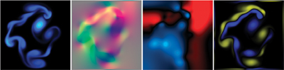
Figure 38-4 The State Fields of a Fluid Simulation, Stored in Textures
Loop Bodies = Fragment Programs
A CPU implementation of the simulation performs the steps in the algorithm by looping, using a pair of nested loops to iterate over each cell in the grid. At each cell, the same computation is performed. GPUs do not have the capability to perform this inner loop over each texel in a texture. However, the fragment pipeline is designed to perform identical computations at each fragment. To the programmer, it appears as if there is a processor for each fragment, and that all fragments are updated simultaneously. In the parlance of parallel programming, this model is known as single instruction, multiple data (SIMD) computation. Thus, the GPU analog of computation inside nested loops over an array is a fragment program applied in SIMD fashion to each fragment.
Feedback = Texture Update
In Section 38.2.4, we described how we use Jacobi iteration to solve Poisson equations. This type of iterative method uses the result of an iteration as input for the next iteration. This feedback is common in numerical methods. In a CPU implementation, one typically does not even consider feedback, because it is trivially implemented using variables and arrays that can be both read and written. On the GPU, though, the output of fragment processors is always written to the frame buffer. Think of the frame buffer as a two-dimensional array that cannot be directly read. There are two ways to get the contents of the frame buffer into a texture that can be read:
- Copy to texture (CTT) copies from the frame buffer to a texture.
- Render to texture (RTT) uses a texture as the frame buffer so the GPU can write directly to it.
CTT and RTT function equally well, but have a performance trade-off. For the sake of generality we do not assume the use of either and refer to the process of writing to a texture as a texture update.
Earlier we mentioned that, in practice, each of the five steps in the algorithm updates a temporary grid and then performs a swap. RTT requires the use of two textures to implement feedback, because the results of rendering to a texture while it is bound for reading are undefined. The swap in this case is merely a swap of texture IDs. The performance cost of RTT is therefore constant. CTT, on the other hand, requires only one texture. The frame buffer acts as a temporary grid, and a swap is performed by copying the data from the frame buffer to the texture. The performance cost of this copy is proportional to the texture size.
38.3.2 Slab Operations
We break down the steps of our simulation into what we call slab operations (slabop, for short). [2] Each slabop consists of processing one or more (often all) fragments in the frame buffer—usually with a fragment program active—followed by a texture update. Fragment processing is driven by rendering geometric primitives. For this application, the geometry we render is simple: just quad and line primitives.
There are two types of fragments to process in any slab operation: interior fragments and boundary fragments. Our 2D grid reserves a single-cell perimeter to store and compute boundary conditions. Typically, a different computation is performed on the interior and at the boundaries. To update the interior fragments, we render a quadrilateral that covers all but a one-pixel border on the perimeter of the frame buffer. We render four line primitives to update the boundary cells. We apply separate fragment programs to interior and border fragments. See Figure 38-5.
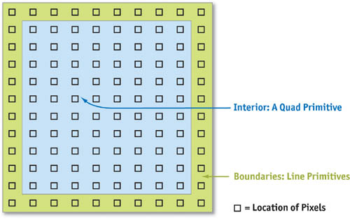
Figure 38-5 Primitives Used to Update the Interior and Boundaries of the Grid
38.3.3 Implementation in Fragment Programs
Now that we know the steps of our algorithm, our data representation, and how to perform a slab operation, we can write the fragment programs that perform computations at each cell.
Advection
The fragment program implementation of advection shown in Listing 38-1 follows nearly exactly from Equation 13, repeated here:

There is one slight difference. Because texture coordinates are not in the same units as our simulation domain (the texture coordinates are in the range [0, N], where N is the grid resolution), we must scale the velocity into grid space. This is reflected in Cg code with the multiplication of the local velocity by the parameter rdx, which represents the reciprocal of the grid scale x. The texture wrap mode must be set to CLAMP_TO_EDGE so that back-tracing outside the range [0, N] will be clamped to the boundary texels. The boundary conditions described later correctly update these texels so that this situation operates correctly.
Example 38-1. Advection Fragment Program
void advect(float2 coords
            : WPOS,
              // grid coordinates
              out float4 xNew
            : COLOR,
              // advected qty
              uniform float timestep, uniform float rdx,
              // 1 / grid scale
              uniform samplerRECT u,
              // input velocity
              uniform samplerRECT x)
// qty to advect
{
  // follow the velocity field "back in time"
  float2 pos = coords - timestep * rdx * f2texRECT(u, coords);
  // interpolate and write to the output fragment
  xNew = f4texRECTbilerp(x, pos);
}
In this code, the parameter u is the velocity field texture, and x is the field that is to be advected. This could be the velocity or another quantity, such as dye concentration. The function f4texRECTbilerp() is a utility to perform bilinear interpolation of the four texels closest to the texture coordinates passed to it. Because current GPUs do not support automatic bilinear interpolation in floating-point textures, we must implement it with this type of code.
Viscous Diffusion
With the description of the Jacobi iteration technique given in Section 38.2.4, writing a Jacobi iteration fragment program is simple, as shown in Listing 38-2.
Example 38-2. The Jacobi Iteration Fragment Program Used to Solve Poisson Equations
void jacobi(half2 coords
            : WPOS,
              // grid coordinates
              out half4 xNew
            : COLOR,
              // result
              uniform half alpha, uniform half rBeta,
              // reciprocal beta
              uniform samplerRECT x,
              // x vector (Ax = b)
              uniform samplerRECT b)
// b vector (Ax = b)
{
  // left, right, bottom, and top x samples
  half4 xL = h4texRECT(x, coords - half2(1, 0));
  half4 xR = h4texRECT(x, coords + half2(1, 0));
  half4 xB = h4texRECT(x, coords - half2(0, 1));
  half4 xT = h4texRECT(x, coords + half2(0, 1));
  // b sample, from center
  half4 bC = h4texRECT(b, coords);
  // evaluate Jacobi iteration
  xNew = (xL + xR + xB + xT + alpha * bC) * rBeta;
}
Notice that the rBeta parameter is the reciprocal of from Equation 16. To solve the diffusion equation, we set alpha to (x)2/t, rBeta to 1/(4 + (x)2/t), and the x and b parameters to the velocity texture. We then run a number of iterations (usually 20 to 50, but more can be used to reduce the error).
Force Application
The simplest step in our algorithm is computing the acceleration caused by external forces. In the demonstration application found in the accompanying materials, you can apply an impulse to the fluid by clicking and dragging with the mouse. To implement this, we draw a spot into the velocity texture at the position of the click. The color of the spot encodes the direction and magnitude of the impulse: the red channel contains the magnitude in x, and the green channel contains the magnitude in y. The spot is actually a two-dimensional Gaussian "splat."
We use a fragment program to check each fragment's distance from the impulse position. Then we add the quantity c to the color:
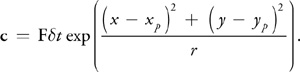
Here, F is the force computed from the direction and length of the mouse drag, is the desired impulse radius, and (x, y) and (xp , yp ) are the fragment position and impulse (click) position in window coordinates, respectively.
Projection
In the beginning of this section, we learned that the projection step is divided into two operations: solving the Poisson-pressure equation for p, and subtracting the gradient of p from the intermediate velocity field. This requires three fragment programs: the aforementioned Jacobi iteration program, a program to compute the divergence of the intermediate velocity field, and a program to subtract the gradient of p from the intermediate velocity field.
The divergence program shown in Listing 38-3 takes the intermediate velocity field as parameter w and one-half of the reciprocal of the grid scale as parameter halfrdx, and it computes the divergence according to the finite difference formula given in Table 38-1, on page 643.
The divergence is written to a temporary texture, which is then used as input to the b parameter of the Jacobi iteration program. The x parameter of the Jacobi program is set to the pressure texture, which is first cleared to all zero values (in other words, we are using zero as our initial guess for the pressure field). The alpha and rBeta parameters are set to -(x)2 and ¼, respectively.
To achieve good convergence on the solution, we typically use 40 to 80 Jacobi iterations. Changing the number of Jacobi iterations will affect the accuracy of the simulation. It is not a good idea to go below 20 iterations, because the error is noticeable. Using more iterations results in more detailed vortices and more overall accuracy, but it requires more computation time. After the Jacobi iterations are finished, we bind the pressure field texture to the parameter p in the following program, which computes the gradient of p according to the definition in Table 38-1 and subtracts it from the intermediate velocity field texture in parameter w. See Listing 38-4.
Example 38-3. The Divergence Fragment Program
void divergence(half2 coords
                : WPOS,
                  // grid coordinates
                  out half4 div
                : COLOR,
                  // divergence
                  uniform half halfrdx,
                  // 0.5 / gridscale
                  uniform samplerRECT w)
// vector field
{
  half4 wL = h4texRECT(w, coords - half2(1, 0));
  half4 wR = h4texRECT(w, coords + half2(1, 0));
  half4 wB = h4texRECT(w, coords - half2(0, 1));
  half4 wT = h4texRECT(w, coords + half2(0, 1));
  div = halfrdx * ((wR.x - wL.x) + (wT.y - wB.y));
}
Example 38-4. The Gradient Subtraction Fragment Program
void gradient(half2 coords
              : WPOS,
                // grid coordinates
                out half4 uNew
              : COLOR,
                // new velocity
                uniform half halfrdx,
                // 0.5 / gridscale
                uniform samplerRECT p,
                // pressure
                uniform samplerRECT w)
// velocity
{
  half pL = h1texRECT(p, coords - half2(1, 0));
  half pR = h1texRECT(p, coords + half2(1, 0));
  half pB = h1texRECT(p, coords - half2(0, 1));
  half pT = h1texRECT(p, coords + half2(0, 1));
  uNew = h4texRECT(w, coords);
  uNew.xy -= halfrdx * half2(pR - pL, pT - pB);
}
Boundary Conditions
In Section 38.2.4, we determined that our "fluid in a box" requires no-slip (zero) velocity boundary conditions and pure Neumann pressure boundary conditions. In Section 38.3.2 we learned that we can implement boundary conditions by reserving the one-pixel perimeter of our grid for storing boundary values. We update these values by drawing line primitives over the border, using a fragment program that sets the values appropriately.
First we should look at how our grid discretization affects the computation of boundary conditions. The no-slip condition dictates that velocity equals zero on the boundaries, and the pure Neumann pressure condition requires the normal pressure derivative to be zero at the boundaries. The boundary is defined to lie on the edge between the boundary cell and its nearest interior cell, but grid values are defined at cell centers. Therefore, we must compute boundary values such that the average of the two cells adjacent to any edge satisfies the boundary condition.
For the velocity boundary on the left side, for example, we have:
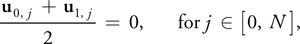
where N is the grid resolution. In order to satisfy this equation, we must set u 0, j equal to –u 1, j . The pressure equation works out similarly. Using the forward difference approximation of the derivative, we get:
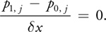
On solving this equation for p 0, j , we see that we need to set each pressure boundary value to the value just inside the boundary.
We can use a simple fragment program for both the pressure and the velocity boundaries, as shown in Listing 38-5.
Example 38-5. The Boundary Condition Fragment Program
void boundary(half2 coords
              : WPOS,
                // grid coordinates
                half2 offset
              : TEX1,
                // boundary offset
                out half4 bv
              : COLOR,
                // output value
                uniform half scale,
                // scale parameter
                uniform samplerRECT x)
// state field
{
  bv = scale * h4texRECT(x, coords + offset);
}
Figure 38-6 demonstrates how this program works. The x parameter represents the texture (velocity or pressure field) from which we read interior values. The offset parameter contains the correct offset to the interior cells adjacent to the current boundary. The coords parameter contains the position in texture coordinates of the fragment being processed, so adding offset to it addresses a neighboring texel. At each boundary, we set offset to adjust our texture coordinates to the texel just inside the boundary. For the left boundary, we set it to (1, 0), so that it addresses the texel just to the right; for the bottom boundary, we use (0, 1); and so on. The scale parameter can be used to scale the value we copy to the boundary. For velocity boundaries, scale is set to -1, and for pressure it is set to 1, so that we correctly implement Equations 17 and 18, respectively.
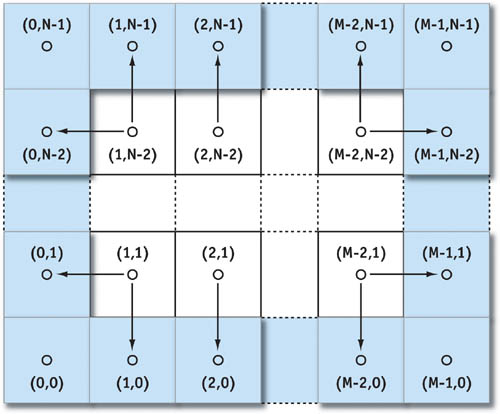
Figure 38-6 Boundary Conditions on an MxN Grid
38.4 Applications
In this section we explore a variety of applications of the GPU simulation techniques discussed in this chapter.
38.4.1 Simulating Liquids and Gases
The most direct use of the simulation techniques is to simulate a continuous volume of a liquid or gas. As it stands, the simulation represents only the velocity of the fluid, which is not very interesting. It is more interesting if we put something else in the fluid. The demonstration application does this by maintaining an additional scalar field. This field represents the concentration of dye carried by the fluid. (Because it is an RGB texture, it is really three scalar fields: one for each of three dye colors.) Quantities like this are known as passive scalars because they are only carried along by the fluid; they do not affect how it flows.
If d is the concentration of dye, then the evolution of the dye field is governed by the following equation:
To simulate how the dye is carried by the fluid, we apply the advection operator to the scalar field, just as we do for the velocity. If we also want to account for the diffusion of the dye in the fluid, we add a diffusion term:
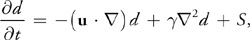
where is the coefficient of the diffusion of dye in water (or whatever liquid we assume the fluid is). To implement dye diffusion, we use Jacobi iteration, just as we did for viscous diffusion of velocity. Note that the demonstration application does not actually perform diffusion of the dye, because numerical error in the advection term causes it to diffuse anyway. We added another term to Equation 20, S. This term represents any sources of dye. The application implements this term by adding dye anywhere we click.
38.4.2 Buoyancy and Convection
Temperature is an important factor in the flow of many fluids. Convection currents are caused by the changes in density associated with temperature changes. These currents affect our weather, our oceans and lakes, and even our coffee. To simulate these effects, we need to add buoyancy to our simulation.
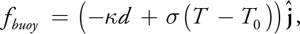
The simplest way to incorporate buoyancy is to add a new scalar field for temperature, T, to the simulation. We can then insert an additional buoyancy operator that adds force where the local temperature is higher than a given ambient temperature, T 0:
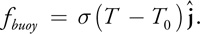
In this equation,
is the vertical direction and s is a constant scale factor. This force can be implemented in a simple
fragment program that evaluates Equation 21 at each fragment, scales the result by the time step, and adds it to
the current velocity.
Smoke and Clouds
We now have almost everything we need to simulate smoke. What we have presented so far is similar to the smoke simulation technique introduced by Fedkiw et al. 2001. In addition to calculating the velocity and pressure fields, a smoke simulation must maintain scalar fields for smoke density, d, and temperature, T. The smoke density is advected by the velocity field, just like the dye we described earlier. The buoyant force is modified to account for the gravitational pull on dense smoke:
where k is a constant mass scale factor.
By adding a source of smoke density and temperature (possibly representing a smokestack or the tip of a cigarette) at a given location on the grid, we simulate smoke. The paper by Fedkiw et al. describes two other differences from our basic simulation. They use a staggered grid to improve accuracy, and they add a vorticity confinement force to increase the amount of swirling motion in the smoke. Both extensions are discussed in the next section.
As demonstrated in Harris et al. 2003, a more complex simulation can be used to simulate clouds on the GPU. A sequence of stills from a 2D GPU cloud simulation is shown in Figure 38-7. The cloud simulator combines fluid simulation with a thermodynamic simulation (including buoyancy), as well as a simulation of water condensation and evaporation. A 128x128 cloud simulation runs at over 80 iterations per second on an NVIDIA GeForce FX 5950 Ultra GPU.
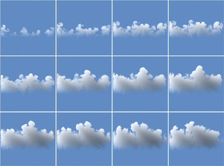
Figure 38-7 Cloud Simulation
38.5 Extensions
The fluid simulation presented in this chapter is a building block that can serve as the basis for more complex simulations. There are many ways to extend this basic simulation. To get you started, we describe some useful extensions.
38.5.1 Vorticity Confinement
The motion of smoke, air and other low-viscosity fluids typically contains rotational flows at a variety of
scales. This rotational flow is vorticity. As Fedkiw et al. explained, numerical dissipation caused by
simulation on a coarse grid damps out these interesting features (Fedkiw et al. 2001). Therefore, they used
vorticity confinement to restore these fine-scale motions. Vorticity confinement works by first
computing the vorticity, =
x
u. From the vorticity we compute a normalized vorticity vector field:

Here,
 The vectors in this vector field point from areas of lower vorticity to areas of higher vorticity. From these
vectors we compute a force that can be used to restore an approximation of the dissipated vorticity:
The vectors in this vector field point from areas of lower vorticity to areas of higher vorticity. From these
vectors we compute a force that can be used to restore an approximation of the dissipated vorticity:
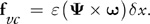
Here
 is a user-controlled scale parameter. The "curl" operator,
x,
can be derived using the definitions of the gradient and the cross-product operator. The accompanying source
code implements vorticity confinement.
is a user-controlled scale parameter. The "curl" operator,
x,
can be derived using the definitions of the gradient and the cross-product operator. The accompanying source
code implements vorticity confinement.
38.5.2 Three Dimensions
All the simulations presented in this chapter are two-dimensional. There is nothing preventing us from extending them to 3D. The equations remain essentially the same, but we must extend them to incorporate a 3D velocity, u = (u, v, w). The fragment programs must be rewritten to account for this; samples from four neighbors in two dimensions become samples from six neighbors in three dimensions.
The biggest change is in how the vector and scalar fields are represented. One option is to use 3D textures. This is a problem on hardware that does not support 3D floating-point textures. In this situation, we can tile the slabs of a 3D texture in a grid stored in a 2D texture (for example, a 32x32x32 grid would tile onto a 256x128 2D texture, with eight tiles in one dimension and four in the other). This technique, called flat 3D textures, is presented in detail in Harris et al. 2003.
38.5.3 Staggered Grid
In our simulation we represent velocity, pressure, and any other quantities at cell centers. This is just one way to discretize the continuous domain on which we represent our fluid. This approach is known as a collocated, or cell-centered, discretization. Another way is to use a staggered grid. In a staggered grid, we represent scalar quantities (such as pressure) at cell centers and vector quantities (such as velocity) at the boundaries between cells. Specifically, on a two-dimensional grid, we represent the horizontal velocity, u, at the right edge of each cell and the vertical velocity, v, at the top edge of each cell. The staggered grid discretization increases the accuracy of many calculations. It can also reduce numerical oscillations that may arise when forces such as buoyancy are applied on a cell-centered grid. Details of the implementation of fluid simulation on a staggered grid can be found in Griebel et al. 1998.
38.5.4 Arbitrary Boundaries
So far we have assumed that our fluid exists in a rectangular box with flat, solid sides. If boundaries of arbitrary shape and location are important, you need to extend the simulation.
Incorporating arbitrary boundaries requires applying the boundary conditions (discussed in Section 38.3.3) at arbitrary locations. This means that at each cell, we must determine in which direction the boundaries lie in order to compute the correct boundary values. This simulation requires more decisions to be made at each cell, leading to a slower and more complicated simulation. However, many interesting effects can be created this way, such as smoke flowing around obstacles. Moving boundaries can even be incorporated, as in Fedkiw et al. 2001. We refer you to that paper as well as Griebel et al. 1998 for implementation details.
38.5.5 Free Surface Flow
Another assumption we made is that our fluid is continuous—the only boundaries we represent are the solid boundaries of the box. So we cannot simulate things like the ocean surface, where there is an interface between the water and air. This type of interface is called a free surface. Extending our simulation to incorporate a free surface requires tracking the location of the surface as it moves through cells. Methods for implementing free surface flow can be found in Griebel et al. 1998.
38.6 Conclusion
The power and programmability now available in GPUs enables fast simulation of a wide variety of phenomena. Underlying many of these phenomena is the dynamics of fluid motion.
After reading this chapter, you should have a fundamental understanding of the mathematics and technology you need to implement basic fluid simulations on the GPU. From these initial ideas you can experiment with your own simulation concepts and incorporate fluid simulation into graphics applications. We hope these techniques become powerful new tools in your repertoire.
38.7 References
Bolz, J., I. Farmer, E. Grinspun, and P. Schröder. 2003. "Sparse Matrix Solvers on the GPU: Conjugate Gradients and Multigrid." In Proceedings of SIGGRAPH 2003.
Chorin, A.J., and J.E. Marsden. 1993. A Mathematical Introduction to Fluid Mechanics. 3rd ed. Springer.
Fedkiw, R., J. Stam, and H.W. Jensen. 2001. "Visual Simulation of Smoke." In Proceedings of SIGGRAPH 2001.
Golub, G.H., and C.F. Van Loan. 1996. Matrix Computations. 3rd ed. The Johns Hopkins University Press.
Goodnight, N., C. Woolley, G. Lewin, D. Luebke, and G. Humphreys. 2003. "A Multigrid Solver for Boundary Value Problems Using Programmable Graphics Hardware." In Proceedings of the SIGGRAPH/Eurographics Workshop on Graphics Hardware 2003.
Griebel, M., T. Dornseifer, and T. Neunhoeffer. 1998. Numerical Simulation in Fluid Dynamics: A Practical Introduction. Society for Industrial and Applied Mathematics.
Harris, M.J., W.V. Baxter, T. Scheuermann, and A. Lastra. 2003. "Simulation of Cloud Dynamics on Graphics Hardware." In Proceedings of the SIGGRAPH/Eurographics Workshop on Graphics Hardware 2003.
Krüger, J., and R. Westermann. 2003. "Linear Algebra Operators for GPU Implementation of Numerical Algorithms." In Proceedings of SIGGRAPH 2003.
Stam, J. 1999. "Stable Fluids." In Proceedings of SIGGRAPH 1999.
Copyright
Many of the designations used by manufacturers and sellers to distinguish their products are claimed as trademarks. Where those designations appear in this book, and Addison-Wesley was aware of a trademark claim, the designations have been printed with initial capital letters or in all capitals.
The authors and publisher have taken care in the preparation of this book, but make no expressed or implied warranty of any kind and assume no responsibility for errors or omissions. No liability is assumed for incidental or consequential damages in connection with or arising out of the use of the information or programs contained herein.
The publisher offers discounts on this book when ordered in quantity for bulk purchases and special sales. For more information, please contact:
U.S. Corporate and Government Sales
(800) 382-3419
corpsales@pearsontechgroup.com
For sales outside of the U.S., please contact:
International Sales
international@pearsoned.com
Visit Addison-Wesley on the Web: www.awprofessional.com
Library of Congress Control Number: 2004100582
GeForce™ and NVIDIA Quadro® are trademarks or registered trademarks of NVIDIA Corporation.
RenderMan® is a registered trademark of Pixar Animation Studios.
"Shadow Map Antialiasing" © 2003 NVIDIA Corporation and Pixar Animation Studios.
"Cinematic Lighting" © 2003 Pixar Animation Studios.
Dawn images © 2002 NVIDIA Corporation. Vulcan images © 2003 NVIDIA Corporation.
Copyright © 2004 by NVIDIA Corporation.
All rights reserved. No part of this publication may be reproduced, stored in a retrieval system, or transmitted, in any form, or by any means, electronic, mechanical, photocopying, recording, or otherwise, without the prior consent of the publisher. Printed in the United States of America. Published simultaneously in Canada.
For information on obtaining permission for use of material from this work, please submit a written request to:
Pearson Education, Inc.
Rights and Contracts Department
One Lake Street
Upper Saddle River, NJ 07458
Text printed on recycled and acid-free paper.
5 6 7 8 9 10 QWT 09 08 07
5th Printing September 2007
- Contributors
- Copyright
- Foreword
- Part I: Natural Effects
-
- Chapter 1. Effective Water Simulation from Physical Models
- Chapter 2. Rendering Water Caustics
- Chapter 3. Skin in the "Dawn" Demo
- Chapter 4. Animation in the "Dawn" Demo
- Chapter 5. Implementing Improved Perlin Noise
- Chapter 6. Fire in the "Vulcan" Demo
- Chapter 7. Rendering Countless Blades of Waving Grass
- Chapter 8. Simulating Diffraction
- Part II: Lighting and Shadows
-
- Chapter 9. Efficient Shadow Volume Rendering
- Chapter 10. Cinematic Lighting
- Chapter 11. Shadow Map Antialiasing
- Chapter 12. Omnidirectional Shadow Mapping
- Chapter 13. Generating Soft Shadows Using Occlusion Interval Maps
- Chapter 14. Perspective Shadow Maps: Care and Feeding
- Chapter 15. Managing Visibility for Per-Pixel Lighting
- Part III: Materials
- Part IV: Image Processing
- Part V: Performance and Practicalities
-
- Chapter 28. Graphics Pipeline Performance
- Chapter 29. Efficient Occlusion Culling
- Chapter 30. The Design of FX Composer
- Chapter 31. Using FX Composer
- Chapter 32. An Introduction to Shader Interfaces
- Chapter 33. Converting Production RenderMan Shaders to Real-Time
- Chapter 34. Integrating Hardware Shading into Cinema 4D
- Chapter 35. Leveraging High-Quality Software Rendering Effects in Real-Time Applications
- Chapter 36. Integrating Shaders into Applications
- Part VI: Beyond Triangles
- Preface