GPU Gems

GPU Gems is now available, right here, online. You can purchase a beautifully printed version of this book, and others in the series, at a 30% discount courtesy of InformIT and Addison-Wesley.

The CD content, including demos and content, is available on the web and for download.

Chapter 23. Depth of Field: A Survey of Techniques

Joe Demers
NVIDIA

23.1 What Is Depth of Field?

Depth of field is the effect in which objects within some range of distances in a scene appear in focus, and objects nearer or farther than this range appear out of focus. Depth of field is frequently used in photography and cinematography to direct the viewer's attention within the scene, and to give a better sense of depth within a scene. In this chapter, I refer to the area beyond this focal range as the background, the area in front of this range as the foreground, and the area in focus as the midground.

The depth-of-field effect arises from the physical nature of lenses. A camera lens (or the lens in your eye) allows light to pass through to the film (or to your retina). In order for that light to converge to a single point on the film (or your retina), its source needs to be a certain distance away from the lens. The plane at this distance from the lens is called the plane in focus. Anything that's not at this exact distance projects to a region (instead of to a point) on the film. This region is known as the circle of confusion (CoC). The diameter of the CoC increases with the size of the lens and the distance from the plane in focus. Because there is a range of distances within which the CoC is smaller than the resolution of the film, photographers and cinematographers refer to this range as being in focus; anything outside of this range is called out of focus. See Figures 23-1 and 23-2.

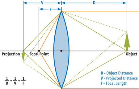
Figure 23-1 A Thin Lens

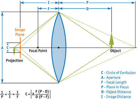
Figure 23-2 The Circle of Confusion

In computer graphics, we typically project onto our virtual film using an idealized pinhole camera that has a lens of zero size, so there is only a single path for light to travel from the scene to the film. So to achieve the depth-of-field effect, we must approximate the blur that would otherwise happen with a real lens.

23.1.1 Calculating the Circle of Confusion

The circle of confusion for the world-space distance from the camera-object distance can be calculated from camera parameters:

 CoC = abs(aperture * (focallength * (objectdistance - planeinfocus)) /           (objectdistance * (planeinfocus - focallength)))

Object distance can be calculated from the z values in the z-buffer:

 objectdistance = -zfar * znear / (z * (zfar - znear) - zfar)

The circle of confusion can alternatively be calculated from the z-buffer values, with the camera parameters lumped into scale and bias terms:

 CoC = abs(z * CoCScale + CoCBias)

The scale and bias terms are calculated from the camera parameters:

 CoCScale = (aperture * focallength * planeinfocus * (zfar - znear)) /              ((planeinfocus - focallength) * znear * zfar) CoCBias = (aperture * focallength * (znear - planeinfocus)) /             ((planeinfocus * focallength) * znear)

23.1.2 Major Techniques

This chapter reviews five main techniques that approximate the depth-of-field effect:

Distributing traced rays across the surface of a (nonpinhole) lens (Cook et al. 1984)
Rendering from multiple cameras—also called the accumulation-buffer technique (Haeberli and Akeley 1990)
Rendering multiple layers (Scofield 1994)
Forward-mapped z-buffer techniques (Potmesil and Chakravarty 1981)
Reverse-mapped z-buffer techniques (Arce and Wloka 2002, Demers 2003)

We spend the most time on the z-buffer techniques, because the others are already well known and have ample coverage in computer graphics literature, and because z-buffer techniques are more amenable to rendering in real time on current graphics hardware.

23.2 Ray-Traced Depth of Field

One use of distributed ray tracing is to render accurate depth of field by casting rays from across the lens, rather than from a single point. With appropriate statistical distribution across the lens, you can achieve the most accurate depth-of-field renderings possible, because you are actually modeling the light transport for the camera and the scene. Although processing time is nowhere near real time, ray-tracing depth of field yields the best quality images. Even when fewer rays are used, the technique degrades nicely to noise, rather than more-objectionable artifacts such as banding or ghosting. It also accommodates effects such as motion blur and soft shadows better than other techniques, due to the ability to jitter samples in time and space independent of neighboring pixels. Figure 23-3 shows an example of this technique and illustrates how noise can occur when too few samples are used.

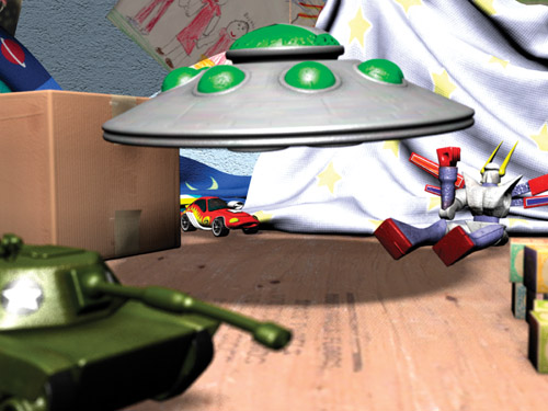
Figure 23-3 Ray-Traced Depth of Field

23.3 Accumulation-Buffer Depth of Field

The accumulation-buffer technique approximates the distributed ray-tracing approach using a traditional z-buffer, along with an auxiliary buffer called an accumulation buffer. An accumulation buffer is a higher precision color buffer that is typically used for accumulating multiple images in real-time rendering.

Whereas distributed ray tracing would cast rays through multiple locations through the lens into the scene, in this technique, we instead render the scene multiple times from different locations through the lens, and then we blend the results using the accumulation buffer. The more rendering passes blended, the better this technique looks, and the closer to "true" depth of field we can get. If too few passes are blended, then we begin to see ghosting, or copies of objects, in the most blurred regions: the extreme foreground and background. The number of passes required is proportional to the area of the circle of confusion, and so for scenes with nonsubtle depth-of-field effects, a prohibitively large number of passes can be required. A single pass per 4 pixels of the area of the largest CoC yields a typically acceptable depth-of-field effect with only barely visible artifacts, because this limits banding artifacts to, at most, 2x2 pixels. Thus, 50 passes are required for an 8-pixel-radius CoC containing roughly 200 pixels. However, a lower-quality rendering using a pass per nine samples (limiting banding to at most 3x3 pixels) with at most a 6-pixel-radius CoC requires only 12 passes. For integer-valued accumulation buffers, precision can quickly become an issue, yielding banding in the final image.

Figure 23-4 shows banding around the barrel of a toy tank, even with only slight amounts of depth of field in the image.

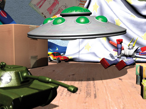
Figure 23-4 Accumulation-Buffer Depth of Field

This is the only potentially real-time technique presented here that can yield "true" depth of field—rendering correct visibility and correct shading from a lens-aperture camera, as opposed to a pinhole camera. Unfortunately, the number of passes typically necessary for good results quickly brings this technique to non-real-time rates.

23.4 Layered Depth of Field

The layered depth-of-field technique is based upon a 2D approach (sometimes called 2½D for the use of layers) that can be performed for simple scenes in 2D paint and photo-editing packages. If objects can be sorted in layers that don't overlap in depth, each layer can be blurred based on some representative depth within its range. These layers can then be composited into a final image to give the impression of depth of field.

23.4.1 Analysis

This technique is simple, and because each layer has a separate image of visible objects, visibility around the edges of objects is treated well. Although the shading is technically incorrect, this tends not to be a noticeable artifact for most scenes.

The downside is that because all pixels within a layer are blurred uniformly, objects that span large depth ranges, especially in the foreground, don't appear to have depth of field within them. Also, the amount of blur can change too quickly between objects that are in front of each other. This happens because their representative depths are based on some average depth of each, rather than the depths of the areas that are close to each other.

Last, many scenes can't be nicely partitioned this way, either because objects partially overlap each others' depth ranges or because objects just span the entire depth range, such as floors and walls. In theory, the scene could be split along planes of equal z, but in practice, a couple of types of artifacts are difficult to overcome. The less-objectionable artifact is that an object split into multiple layers will be blurred differently on either side of that split, and so an artificial edge can become visible within the object. The worse artifact arises from potential errors of visibility due to the splitting along z. Because some objects are split, smaller objects behind them that shouldn't be visible can be blended into the layer. Figure 23-5 shows the constant blur artifact generated when simply rendering a layer for each object. This is especially noticeable in the floor, which is too sharp in the foreground and too blurry in the background.

Figure 23-5 Layered Depth of Field

Because of these artifacts, and the difficulty in resolving them in the general case, this technique tends to be used only in special cases where such problems can be fixed with ad hoc solutions.

23.5 Forward-Mapped Z-Buffer Depth of Field

Using forward mapping (that is, rendering sprites) to approximate depth of field allows for a depth-of-field effect that works for arbitrary scenes. This is the primary method used by post-processing packages to apply depth of field to rendered images and movies. Forward mapping in this case refers to the process of mapping source pixels onto the destination image, as opposed to reverse mapping, which identifies which source pixel needs to be mapped onto the destination image. The idea is to save both the color buffer and the depth buffer when rendering, and then use the depth buffer to determine the CoC for that pixel. The pixels are blended into the frame buffer as circles whose colors are the pixels' colors, whose diameter equals the CoC, and with alpha values inversely proportional to the circles' areas. Pixels blend into only those neighboring pixels farther from the camera than themselves, to avoid blurry pixels affecting sharp pixels in front of them. A final renormalizing pass is typically done to account for pixels whose final alphas don't sum to 1. This is necessary because pixels whose alpha is less than 1 also have colors that are artificially less than the weighted average of their contributors.

23.5.1 Analysis

Because this technique relies only on information from images rendered with a pinhole camera model, it uses incorrect visibility and shading in its calculations. So if a point light is animated passing behind an object, it will transition immediately from visible to not visible, rather than from fully visible, to visible from some parts of the lens, to not visible. For many applications, however, this technique is good enough, and the artifacts can be covered up with lens flares and other artistic patches.

Unfortunately, this technique doesn't map well to hardware, because it relies on rendering millions of sprites (the constant color circles) at typical screen resolutions. In software, special-purpose algorithms keep this reasonably efficient, but still nowhere near real time. Attempts have been made to use variants of these algorithms, by blending the translated source image multiple times with per-pixel weights based upon the CoC of the pixel and the distance translated. However, the same trade-offs apply here as for the layered depth-of-field effect. Although the passes are much simpler geometrically, even more passes are required: typically one per pixel of the largest CoC. Figure 23-6 shows an example of this technique, which worked rather well for this scene—no obvious artifacts are evident.

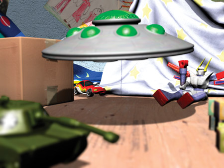
Figure 23-6 Forward-Mapped Z-Buffer Depth of Field

23.6 Reverse-Mapped Z-Buffer Depth of Field

The final technique is the reverse-mapped (that is, texture-mapped) z-buffer technique, which is similar in many ways to the forward-mapping technique. It also works off a color and depth image, but instead of rendering blended sprites onto the screen, this technique blurs the rendered scene by varying amounts per pixel, depending on the depth found in the z-buffer. Each pixel chooses a greater level of blurriness for a larger difference between its z value and the z value of the plane in focus. The ways in which this blurred version is generated and applied account for the main variants of this technique.

The simplest variant allows the hardware to create mipmaps of the scene texture and then performs a texture lookup, specifying the circle of confusion as the derivatives passed along to decide which mip level to read from. See Figures 23-7, 23-8, and 23-9. However, until the release of the GeForce FX and the Radeon 9700, graphics hardware couldn't choose which mip level of a texture to read per pixel.

Figure 23-7 Reverse-Mapped Z-Buffer Depth of Field

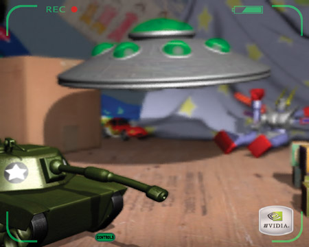
Figure 23-8 Reverse-Mapped Z-Buffer Depth of Field

Figure 23-9 No Depth-of-Field Simulation

Earlier variants of this technique therefore used multiple blurred textures to approximate the blur introduced by depth of field. Some techniques used the same texture bound multiple times with different mip-level biases, and some explicitly created new blurred textures, often with better down-sampling filters (3x3 or 5x5 rather than 2x2). These variants would typically perform three lookups—the original scene, the quarter-sized (¼x¼) texture, and the sixteenth-sized ( x ) texture—and blend between them based upon the pixel's z value. Instead of letting the hardware generate mipmaps, it's also possible to render-to-texture to each mipmap with better filter kernels to get better-quality mipmaps. The hardware's mipmap generation is typically faster, however, so this becomes a bit of a quality/performance trade-off. Another interesting variant uses the hardware to generate a floating-point summed-area table for the color texture instead of mipmaps. Although the use of summed-area tables fixes the bilinear interpolation artifacts discussed later, this technique is quite a bit slower, and it actually isn't guaranteed to produce well-defined results.

Unfortunately, the technique used to build the summed-area table renders to the same texture it's reading from, rendering vertical lines to sum horizontally, and horizontal lines to sum vertically. Reading from the same texture being written isn't guaranteed to produce well-defined results using current graphics APIs (that is, the API allows the graphics driver to draw black, garbage, or something else rather than the expected result). It has been tested, and it does work on current hardware and drivers in OpenGL, but this could change with new hardware or a new version of the driver.

23.6.1 Analysis

Although this technique is in general significantly faster than other techniques, it has a variety of limitations. Some of these are minor and exist in many of the other techniques, but some are more objectionable and are unique to this technique alone.

Artifacts Due to Depth Discontinuities

The most objectionable artifact is caused by depth discontinuities in the depth image. Because only a single z value is read to determine how much to blur the image (that is, which mip level to choose), a foreground (blurry) object won't blur out over midground (sharp) objects. See Figure 23-10. One solution is to read multiple depth values, although unless you can read a variable number of depth values, you will have a halo effect of decreasing blur of fixed radius, which is nearly as objectionable as the depth discontinuity itself. Another solution is to read a blurred depth buffer, but this causes artifacts that are just as objectionable: blurring along edges of sharp objects and sharpening along edges of blurry objects. Extra blur can be added to the whole scene by uniformly biasing the calculated CoC. Adding a little extra blur when the focal plane moved too close (and not letting the focal plane move too close too often) helped hide this artifact fairly well in the GeForce FX launch demo, "Toys," from which the images in this chapter were taken.

Figure 23-10 Depth Discontinuity Artifacts

Artifacts Due to Bilinear Interpolation

The magnification of the smaller mipmaps or blurred images results in bilinear interpolation artifacts. See Figure 23-11. This problem has some easier solutions, including using the summed-area tables approach, using the multiple blurred images approach with full-sized images (rather than down-sampling), or jittering the sampling position (potentially with multiple samples) proportional to the CoC in the mipmap approach. See Figure 23-12.

Figure 23-11 Magnification Artifacts with Trilinear Filtering

Figure 23-12 Noise Artifacts with Jittered Trilinear Filtering

In the "Toys" demo, we used the jittered mipmap sample approach because it was the fastest. Although the jittering introduces artifacts of its own, the noise produced was preferable to the crawling, square, stair-stepping patterns of the non-jittered version, especially during animation.

Artifacts Due to Pixel Bleeding

The least objectionable artifact is pixel bleeding. Because the color image is blurred indiscriminately, areas in focus can incorrectly bleed into nearby areas out of focus. In a typical scene, this problem tends not to be very noticeable, but it's easy to build atypical situations where it becomes quite apparent. See Figure 23-13.

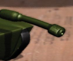
Figure 23-13 Pixel-Bleeding Artifacts

One solution is to render separate objects into layers, perform the reverse-mapped z-buffer depth-of-field technique on each separately, and then composite them together. This doesn't completely solve the problem. However, it resolves the common cases, because individual objects tend to have a similar color scheme internally, and they tend not to overlap themselves by large differences in depth. This can also reduce the effect of depth discontinuities if the clear depth for each layer is set to the farthest depth within the layer. Typically, if the layer's object is out of focus, this clear depth will also be out of focus, and so this object will blur out over objects behind it. There will generally be some discontinuity, but it will tend to be lessened by this technique. However, as in the layered depth-of-field technique, this layer sorting can be used only for certain scenes.

23.7 Conclusion

In this chapter, we've examined the major depth-of-field techniques, along with their benefits and problems. Unfortunately, no single depth-of-field algorithm meets everyone's quality and speed requirements. When correct shading is necessary but real-time processing isn't, the ray-traced or accumulation-buffer depth-of-field algorithms are the appropriate choices. When speed is of utmost importance, the layered or z-buffer depth-of-field algorithms are a better choice. For post-processing rendered scenes, the best quality is available through the splatting depth-of-field technique.

We've examined the z-buffer depth-of-field algorithm in detail, because there isn't a canonical paper in the literature, as there is for the other techniques, and because it's the one most likely to be useful for truly real-time applications. The pixel-bleeding artifact is the hardest to fix, but fortunately it is also the least objectionable. The bilinear interpolation artifacts are fairly easily solved, with some performance cost, by better filtering between mipmaps or textures. Last, the most objectionable artifacts due to depth discontinuities are only really solved by avoiding those cases in which they occur (that is, when the focal plane is far into the scene), which limits the utility of the algorithm for general purposes but is good enough for many real-time applications.

23.8 References

Arce, Tomas, and Matthias Wloka. 2002. "In-Game Special Effects and Lighting." Available online at http://www.nvidia.com/object/gdc_in_game_special_effects.html

Cant, Richard, Nathan Chia, and David Al-Dabass. 2001 "New Anti-Aliasing and Depth of Field Techniques for Games." Available online at http://ducati.doc.ntu.ac.uk/uksim/dad/webpagepapers/Game-18.pdf

Chen, Y. C. 1987. "Lens Effect on Synthetic Image Generation Based on Light Particle Theory." The Visual Computer 3(3).

Cook, R., T. Porter, and L. Carpenter. 1984. "Distributed Ray Tracing." In Proceedings of the 11th Annual Conference on Computer Graphics and Interactive Techniques.

Demers, Joe. 2003. "Depth of Field in the 'Toys' Demo." From "Ogres and Fairies: Secrets of the NVIDIA Demo Team," presented at GDC 2003. Available online at http://developer.nvidia.com/docs/IO/8230/GDC2003_Demos.pdf

Dudkiewicz, K. 1994. "Real-Time Depth-of-Field Algorithm." In Image Processing for Broadcast and Video Production: Proceedings of the European Workshop on Combined Real and Synthetic Image Processing for Broadcast and Video Production, edited by Yakup Paker and Sylvia Wilbur, pp. 257–268. Springer-Verlag.

Green, Simon. 2003. "Summed Area Tables Using Graphics Hardware." Available online at http://www.opengl.org/resources/tutorials/gdc2003/GDC03_SummedAreaTables.ppt

Haeberli, Paul, and Kurt Akeley. 1990. "The Accumulation Buffer: Hardware Support for High-Quality Rendering." Computer Graphics 24(4). Available online at http://graphics.stanford.edu/courses/cs248-02/haeberli-akeley-accumulation-buffer-sig90.pdf

Krivánek, Jaroslav, Jirí Zára, and Kadi Bouatouch. 2003. "Fast Depth of Field Rendering with Surface Splatting." Presentation at Computer Graphics International 2003. Available online at http://www.cgg.cvut.cz/~xkrivanj/papers/cgi2003/9-3_krivanek_j.pdf

Mulder, Jurriaan, and Robert van Liere. 2000. "Fast Perception-Based Depth of Field Rendering." Available online at http://www.cwi.nl/~robertl/papers/2000/vrst/paper.pdf

Potmesil, Michael, and Indranil Chakravarty. 1981. "A Lens and Aperture Camera Model For Synthetic Image Generation." Computer Graphics.

Potmesil, Michael, and Indranil Chakravarty. 1982. "Synthetic Image Generation with a Lens and Aperture Camera Model." ACM Transactions on Graphics, April 1982.

Rokita, P. 1993. "Fast Generation of Depth of Field Effects in Computer Graphics." Computers & Graphics 17(5), pp. 593–595.

Scofield, Cary. 1994. "2½-D Depth of Field Simulation for Computer Animation." In Graphics Gems III, edited by David Kirk. Morgan Kaufmann.

Copyright

Many of the designations used by manufacturers and sellers to distinguish their products are claimed as trademarks. Where those designations appear in this book, and Addison-Wesley was aware of a trademark claim, the designations have been printed with initial capital letters or in all capitals.

The authors and publisher have taken care in the preparation of this book, but make no expressed or implied warranty of any kind and assume no responsibility for errors or omissions. No liability is assumed for incidental or consequential damages in connection with or arising out of the use of the information or programs contained herein.

The publisher offers discounts on this book when ordered in quantity for bulk purchases and special sales. For more information, please contact:

U.S. Corporate and Government Sales
(800) 382-3419
corpsales@pearsontechgroup.com

For sales outside of the U.S., please contact:

International Sales
international@pearsoned.com

Visit Addison-Wesley on the Web: www.awprofessional.com

Library of Congress Control Number: 2004100582

GeForce™ and NVIDIA Quadro^® are trademarks or registered trademarks of NVIDIA Corporation.
RenderMan^® is a registered trademark of Pixar Animation Studios.
"Shadow Map Antialiasing" © 2003 NVIDIA Corporation and Pixar Animation Studios.
"Cinematic Lighting" © 2003 Pixar Animation Studios.
Dawn images © 2002 NVIDIA Corporation. Vulcan images © 2003 NVIDIA Corporation.

All rights reserved. No part of this publication may be reproduced, stored in a retrieval system, or transmitted, in any form, or by any means, electronic, mechanical, photocopying, recording, or otherwise, without the prior consent of the publisher. Printed in the United States of America. Published simultaneously in Canada.

For information on obtaining permission for use of material from this work, please submit a written request to:

Pearson Education, Inc.
Rights and Contracts Department
One Lake Street
Upper Saddle River, NJ 07458

Text printed on recycled and acid-free paper.

5 6 7 8 9 10 QWT 09 08 07

5th Printing September 2007

Part II: Lighting and Shadows

Part III: Materials

Part IV: Image Processing

Part V: Performance and Practicalities

Part VI: Beyond Triangles

Preface