GPU Gems
GPU Gems is now available, right here, online. You can purchase a beautifully printed version of this book, and others in the series, at a 30% discount courtesy of InformIT and Addison-Wesley.
The CD content, including demos and content, is available on the web and for download.
Chapter 17. Ambient Occlusion
Matt Pharr
NVIDIA
Simon Green
NVIDIA
The real-time computer graphics community has recently started to appreciate the increase in realism that comes from illuminating objects with complex light distributions from environment maps, rather than using a small number of simple light sources. In the real world, light arrives at surfaces from all directions, not from just a handful of directions to a point or directional light sources, and this noticeably affects their appearance. A variety of techniques have recently been developed to capture real-world illumination (such as on movie sets) and to use it to render objects as if they were illuminated by the light from the original environment, making it possible to more seamlessly merge computer graphics with real scenes. For completely synthetic scenes, these techniques can be applied to improve the realism of rendered images by rendering an environment map of the scene and using it to light characters and other objects inside the scene. Rather than using the map just for perfect specular reflection, these techniques use it to compute lighting for glossy and diffuse surfaces as well.
This chapter describes a simple technique for real-time environment lighting. It is limited to diffuse surfaces, but it is efficient enough for real-time use. Furthermore, this method accurately accounts for shadows due to geometry occluding the environment from the point being shaded. Although the shading values that this technique computes have a number of sources of possible errors compared to some of the more complex techniques recently described in research literature, the technique is relatively easy to implement. (To make it work, you don't have to understand and implement a spherical harmonics library!) The approach described here gives excellent results in many situations, and it runs interactively on modern hardware.
This method is based on a view-independent preprocess that computes occlusion information with a ray tracer and then uses this information at runtime to compute a fast approximation to diffuse shading in the environment. This technique was originally developed by Hayden Landis (2002) and colleagues at Industrial Light & Magic; it has been used on a number of ILM's productions (with a non-real-time renderer!).
17.1 Overview
The environment lighting technique we describe has been named ambient occlusion lighting. One way of thinking of the approach is as a "smart" ambient term that varies over the surface of the model according to how much of the external environment can be seen at each point. Alternatively, one can think of it as a diffuse term that supports a complex distribution of incident light efficiently. We will stick with the second interpretation in this chapter.
The basic idea behind this technique is that if we preprocess a model, computing how much of the external environment each point on it can see versus how much of the environment has been occluded by other parts of the model, then we can use that information at rendering time to compute the value of a diffuse shading term. The result is that the crevices of the model are realistically darkened, and the exposed parts of the model realistically receive more light and are thus brighter. The result looks substantially more realistic than if a standard shading model had been used.
This approach can be extended to use environment lighting as the source of illumination, where an environment map that represents incoming light from all directions is used to determine the color of light arriving at each point on the object. For this feature, in addition to recording how much of the environment is visible from points on the model, we also record from which direction most of the visible light is arriving. These two quantities, which effectively define a cone of unoccluded directions out into the scene, can be used together to do an extremely blurred lookup from the environment map to simulate the overall incoming illumination from a cone of directions of interest at a point being shaded.
17.2 The Preprocessing Step
Given an arbitrary model to be shaded, this technique needs to know two things at each point on the model: (1) the "accessibility" at the point—what fraction of the hemisphere above that point is unoccluded by other parts of the model; and (2) the average direction of unoccluded incident light. Figure 17-1 illustrates both of these ideas in 2D. Given a point P on the surface with normal N, here roughly two-thirds of the hemisphere above P is occluded by other geometry in the scene, while one-third is unoccluded. The average direction of incoming light is denoted by B, and it is somewhat to the right of the normal direction N. Loosely speaking, the average color of incident light at P could be found by averaging the incident light from the cone of unoccluded directions around the B vector.
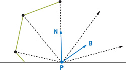
Figure 17-1 Computing Accessibility and an Average Direction
This B vector and the accessibility value, which are model dependent but not lighting dependent, can be computed offline in a preprocess with a ray tracer. For the examples in this chapter, the model we used was finely tessellated, so we computed these values at the center of each triangle and then stored values at each vertex that held the average of the values from the adjacent faces. We then passed these per-vertex values through the vertex shader so that they would be interpolated at each pixel for the fragment shader. Alternatively, we could have stored them in texture maps; this would have been preferable if the model had been more coarsely tessellated.
The pseudocode in Listing 17-1 shows our basic approach. At the center of each triangle, we generate a set of rays in the hemisphere centered about the surface normal. We trace each of these rays out into the scene, recording which of them intersect the model—indicating that we wouldn't receive light from the environment in that direction—and which are unoccluded. We compute the average direction of the unoccluded rays, which gives us an approximation to the average direction of incident light. (Of course, it's possible that the direction that we compute may in fact be occluded itself; we just ignore this issue.)
Example 17-1. Basic Algorithm for Computing Ambient Occlusion Quantities
For each triangle
{
  Compute center of triangle Generate set of rays over the hemisphere there
      Vector avgUnoccluded = Vector(0, 0, 0);
  int numUnoccluded = 0;
  For each ray
  {
If (ray doesn't intersect anything) {
avgUnoccluded += ray.direction;
++numUnoccluded;
  }
}
avgUnoccluded = normalize(avgUnoccluded);
accessibility = numUnoccluded / numRays;
}
An easy way to generate these rays is with rejection sampling: randomly generate rays in the 3D cube from –1 to 1 in x, y, and z, and reject the ones that don't lie in the unit hemisphere about the normal. The directions that survive this test will have the desired distribution. This approach is shown in the pseudocode in Listing 17-2. More complex Monte Carlo sampling algorithms could also be used to ensure a better-distributed set of sample directions.
Example 17-2. Algorithm for Computing Random Directions with Rejection Sampling
while (true)
{
  x = RandomFloat(-1, 1); // random float between -1 and 1
  y = RandomFloat(-1, 1);
  z = RandomFloat(-1, 1);
  if (x * x + y * y + z * z > 1)
    continue; // ignore ones outside unit
  // sphere
  if (dot(Vector(x, y, z), N) < 0)
    continue;
  // ignore "down" dirs
  return normalize(Vector(x, y, z)); // success!
}
17.3 Hardware-Accelerated Occlusion
It is possible to accelerate the calculation of this occlusion information by using the graphics hardware instead of software ray tracing. Shadow maps provide a fast image-space method of determining whether a point is in shadow. (GeForce FX has special hardware support for rasterizing the depth-only images needed for shadow mapping at high speed.) Instead of shooting rays from each point on the surface, we can reverse the problem and surround the object with a large spherical array of shadow-mapped lights. The occlusion amount at a point on a surface is simply the average of the shadow contributions from each light. We can calculate this average using a floating-point accumulation buffer. For n lights, we render the scene n times, each time moving the shadow-casting light to a different position on the sphere. We accumulate these black-and-white images to form the final occlusion image. At the limit, this simulates a large area light covering the sky.
A large number of lights (128 to 1024) is required for good results, but the performance of modern graphics hardware means this technique can still be faster than ray tracing. The distribution of the lights on the sphere also affects the final quality. The most obvious method is to use polar coordinates, with lights distributed at evenly spaced longitudes and latitudes, but this tends to concentrate too many samples at the poles. Instead, you should use a uniform distribution on the sphere. If the object is standing on a ground plane, a full hemisphere of lights isn't necessary—a dome or a hemisphere can be used instead.
Another issue that can affect the quality of the final results is shadow-mapping artifacts. These often appear as streaking on the surface at the transition from lit to shadowed. This problem can be alleviated by multiplying the shadowing term by a function of the normal and the light direction that ensures that the side of the surface facing away from the light is always black.
One disadvantage of this method is that for each light, two passes are required: one to generate the shadow map and one to render the shadowed scene, plus the overhead needed to accumulate the image. For n lights, this means 2n passes are required. It may be faster to accumulate the effect of multiple shadow maps in a single pass. Since current hardware supports eight sets of texture coordinates, it is possible to accumulate eight shadows in the shader at once. This means that only n + n/8 renders of the scene would be required in total.
The approach can also be extended to produce the average unoccluded direction, or bent normal. We can use a shader to calculate the direction to the light multiplied by the shadow value, and then copy the result to the RGB output color. The occlusion information can be stored in the alpha channel. We accumulate these RGB normal values in the same way as the occlusion value, and then we normalize the final result to get the average unoccluded normal. Note that a half (16-bit) floating-point accumulation buffer may not have sufficient precision to represent the summation of these vectors accurately.
So far, the technique we have described generates occlusion images in camera space, but often we want to generate textures that store the occlusion information. If the objects we are using have unique texture coordinates (that is, the texture covers their entire surface without overlaps), this is relatively easy. We can unwrap the model with a vertex program that uses the UV texture coordinate as the screen-space position. The calculation proceeds as normal, but instead of rendering the object as normal, we are rendering the rectangular unwrapped mesh. Once this occlusion texture has been generated, it can be used in real-time rendering, as described in the rest of this chapter.
17.4 Rendering with Ambient Occlusion Maps
As an example, we applied this method to a complex model set on a plane. (There are no texture maps in this scene, so that we can see the effect of the method more clearly. Texturing is easily incorporated into this technique, however.) We used 512 rays per triangle to compute the accessibility values and average unoccluded directions for each of 150,000 triangles; the preprocess took approximately four minutes with a software ray tracer on an AMD Athlon 1800XP CPU. We then wrote this information out to disk in a file for use by our demo application. For comparison, Figure 17-2 shows an image of the model with a simple diffuse shading model light by a point light, with no shadows. Note the classic unrealistic computer graphics appearance and lack of shading complexity. For example, the underside of the creature and the inside of its far leg are both too bright.
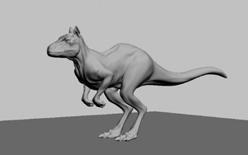
Figure 17-2 Scene Shaded with the Simple Diffuse Shading Model
In Figure 17-3, we shaded the model by setting the color to be the accessibility at each point, as computed by the ray-traced preprocess. Note that crevices under the legs of the model and points on its stomach are darker than exposed regions such as its back, which is almost fully exposed. The harsh transitions from light to dark in Figure 17-2 that were the result of the changing orientation of the surface normal with respect to the point light's position have been smoothed out, giving a realistic "overcast skylight" effect. There is a very soft shadow beneath the creature on the ground plane, the result of the creature's body reducing the amount of light arriving at the points beneath it.
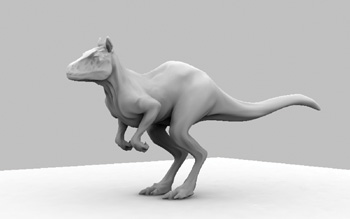
Figure 17-3 Scene Shaded with Accessibility Information
This shadow helps to ground the model, showing that it is in fact on the ground plane, rather than floating above it, as might be the case in Figure 17-2.
Best of all, shading with the accessibility value doesn't even require advanced programmable graphics hardware; it can be done with ancient graphics hardware, just by passing appropriate color values with each vertex of the model. As such, it can run at peak performance over a wide range of GPU architectures. If this model had a diffuse texture map, we'd just multiply the texture value by the accessibility for shading it.
17.4.1 Environment Lighting
If programmable graphics hardware is available, we can use the accessibility information in a more sophisticated way to generate more complex shading effects. Here, we compute an approximation of how the model would appear if it were inside a complex real-world environment, using captured illumination from an environment map of the scene. For this example, we used an environment map of Galileo's tomb, in Florence, shown in Figure 17-4.
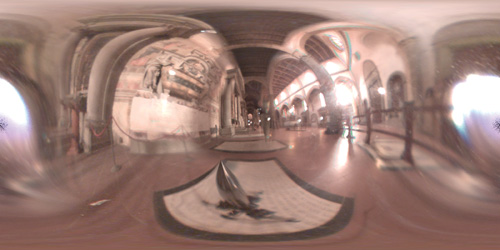
Figure 17-4 An Environment Map of Galileo's Tomb, in Latitude-Longitude Format
This environment map has a different parameterization than the cube maps and sphere maps that are widely used now in interactive graphics. It is known as a lat-long map, for latitude-longitude, because the parameterization is similar to the latitudes and longitudes used to describe locations on Earth. It maps directions to points on the map using the spherical coordinate parameterization of a sphere, where ranges from 0 to vertically and ranges from 0 to 2 horizontally, x = sin cos , y = sin sin , and z = cos . Given a direction (x, y, z), inverting these equations gives a (, ) value, which is mapped to texture coordinates in the map by dividing it by (2, ). We used this type of environment map because it allows us to do extremely blurred lookups without artifacts; unfortunately, blurred cube-map lookups that span multiple faces of the cube are not handled correctly by current hardware.
The basic idea behind the program for shading with such an environment map is this: We would like to use the information that we have so far to compute a good approximation of how much light is arriving at the surface at the point being shaded. The two factors that affect this value are (1) which parts of the hemisphere above the point are unoccluded by geometry between the point and the environment map and (2) what is the incoming light along these directions. Figure 17-5 shows two cases of this scene. On the left, the point being shaded can see only a small fraction of the directions above it, denoted by the direction vector B and the circle indicating a cone of directions; accessibility here is very low. On the right, more light reaches the point, along a greater range of directions.
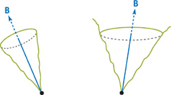
Figure 17-5 Approximating Different Amounts of Visibility
The accessibility value computed in the preprocess tells us what fraction of the hemisphere can see the environment map, and the average visible direction gives us an approximation of the direction around which to estimate the incoming light. Although this direction may point in a direction that is actually occluded (for example, if two separate regions of the hemisphere are unoccluded but the rest are occluded, the average direction may be between the two of them), it usually works well in practice.
The basic fragment shader we used is shown in Listing 17-3. The average direction of incoming light is passed in via the B variable, and the fraction of the hemisphere that was unoccluded is passed in via accessibility; the envlatlong sampler is bound to the environment map in Figure 17-4.
Example 17-3. Fragment Shader for Shading with Accessibility Values and an Environment Map
half4 main(half3 B
           : TEXCOORD0, half accessibility
           : TEXCOORD1, uniform sampler2D envlatlong)
    : COLOR
{
  half2 uv = latlong(B);
  half2 blurx, blury;
  computeBlur(uv, accessibility, blurx, blury);
  half3 Cenv = tex2D(envlatlong, uv, blurx, blury).xyz;
  return half4(accessibility * Cenv, 1);
}
There are three main steps to the shader. First, we call the latlong() function shown in Listing 17-4 to compute the (u, v) texture coordinates in the latitude-longitude environment map. Second, the computeBlur() function, shown in Listing 17-5, determines the area of the map to blur over for the point that we are shading. Finally, we do the blurred environment map lookup via the variant of the tex2D() function that allows us to pass in derivatives. The derivatives specify the area of the map over which to do texture filtering, giving the average light color inside the cone. This is scaled by the accessibility value and returned. Thanks to mipmapping, computing blurred regions of large sections of the environment map can be done very efficiently in the graphics hardware.
Example 17-4. The latlong() Function Definition
#define PI 3.1415926
half2 latlong(half3 v)
{
  v = normalize(v);
  half theta = acos(v.z); // +z is up
  half phi = atan2(v.y, v.x) + PI;
  return half2(phi, theta) * half2(.1591549, .6366198);
}
For clarity, we have listed separately the two subroutines that the fragment shader uses. First is latlong(), which takes a 3D direction and finds the 2D texture position that the direction should map to for the latitude-longitude map. Because the hardware does not support latitude-longitude maps directly, we need to do this computation ourselves.
Example 17-5. The computeBlur() Function Definition
void computeBlur(half2 uv, half accessibility, out half2 blurx, out half2 blury)
{
  half width = sqrt(accessibility);
  blurx = half2(width, 0);
  blury = half2(0, width);
}
However, because inverse trigonometric functions are computationally expensive, in our implementation we stored theta and phi values in a 256x256 cube-map texture with signed eight-bit components and did a single cube-map lookup in place of the entire latlong() function. This modification saved approximately fifty fragment program instructions in the compiled result, with no loss in quality in the final image.
The only other tricky part of this shader is computing how much of the environment map to filter over. (Recall Figure 17-5, where the point on the left receives light from a smaller cone of directions than the point on the right does.) We make a very rough approximation of the area to filter over in the computeBlur() function; it just captures the first-order effect that increased accessibility should lead to an increased filter area.
The result of applying this shader to the model is shown in Figure 17-6. The shader compiles to approximately ten GPU instructions, and the scene renders at real-time rates on modern GPUs.
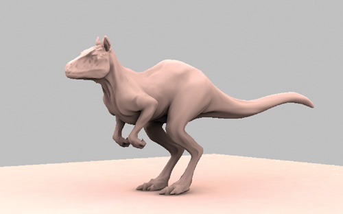
Figure 17-6 Scene Shaded with Accessibility Information and Illumination from an Environment Map
17.5 Conclusion
The environment lighting technique that we describe here employs many approximations, but it works well in practice and has proven itself in rendering for movie effects. The method separates the problem into a relatively expensive preprocess that computes just the right information needed to do fast shading at rendering time. The preprocess does not depend on the lighting environment map, so dynamic illumination from the scene can easily be used. Because a very blurred version of the scene's environment map is used, it doesn't necessarily need to be re-rendered for each frame. The visual appearance of objects shaded with this method is substantially more realistic than if standard graphics lighting models are used.
Texture-mapped surfaces and standard light sources are easily incorporated into this method. Even better results can be had with a small number of standard point or directional lights to cast hard shadows, provide "key" lighting, and generate specular highlights.
While many applications of environment lighting have focused on the advantages of "high-dynamic-range" environment maps (that is, maps with floating-point texel values, thus encoding a wide range of intensities), this method works well even with standard eight-bit-per-channel texture maps. Because it simulates reflection only from diffuse surfaces—it averages illumination over many directions—it's less important to accurately represent bright light from a small set of directions, as is necessary for more glossy reflections.
We have not addressed animation in this chapter. As an animated character model changes from one pose to another, obviously the occlusion over the entire model changes. We believe that computing the occlusion information for a series of reference poses and interpolating between the results according to the character's pose would work well in practice, but we have not implemented this improvement here. However, NVIDIA's "Ogre" demo used this approach successfully. See Figure 17-7.

Figure 17-7 The Ogre Character
17.6 Further Reading
This section describes alternative approaches to environment lighting in more general ways. In particular, ambient occlusion can be understood in the context of spherical harmonic lighting techniques; it is an extreme simplification that uses just the first spherical harmonic to represent reflection.
Landis, Hayden. 2002. "Production-Ready Global Illumination." Course 16 notes, SIGGRAPH 2002. Available online at http://www.renderman.org/RMR/Books/sig02.course16.pdf.gz . Hayden Landis and others at ILM developed the ideas that we have described and implemented in Cg in this chapter. Hayden documented the approach in these notes, and a complete list of the inventors of this shading technique appears at the end.
Zhukov, S., A. Iones, and G. Kronin. 1998. "An Ambient Light Illumination Model." In Proceedings of Eurographics Rendering Workshop '98, pp. 45–56. Zhukov et al. described a similar "smart ambient" method based on a ray-traced preprocess in this article, though they didn't use it for environment lighting.
Blinn, J. F., and Newell, M. E. 1976. "Texture and Reflection in Computer Generated Images." Communications of the ACM 19(10)(October 1976), pp. 542–547. The idea of using environment maps for lighting specular objects was first described in this article.
Miller, Gene S., and C. Robert Hoffman. 1984. "Illumination and Reflection Maps: Simulated Objects in Simulated and Real Environments." Course notes for Advanced Computer Graphics Animation, SIGGRAPH 84. The application to lighting nonspecular objects was first described in these course notes.
Debevec, Paul. 1998. "Rendering Synthetic Objects into Real Scenes: Bridging Traditional and Image-Based Graphics with Global Illumination and High Dynamic Range Photography." In Proceedings of SIGGRAPH 98, pp. 189–198. Interest in environment lighting grew substantially after this paper appeared.
Cohen, Michael, and Donald P. Greenberg. 1985. "The Hemi-Cube: A Radiosity Solution for Complex Environments." This paper was the first to describe the hemi-cube algorithm for radiosity, another approach for the occlusion preprocess that would easily make use of graphics hardware for that step.
A series of recent SIGGRAPH papers by Ramamoorthi and Hanrahan and by Sloan et al. has established key mathematical principles and algorithms based on spherical harmonics for fast environment lighting.
Copyright
Many of the designations used by manufacturers and sellers to distinguish their products are claimed as trademarks. Where those designations appear in this book, and Addison-Wesley was aware of a trademark claim, the designations have been printed with initial capital letters or in all capitals.
The authors and publisher have taken care in the preparation of this book, but make no expressed or implied warranty of any kind and assume no responsibility for errors or omissions. No liability is assumed for incidental or consequential damages in connection with or arising out of the use of the information or programs contained herein.
The publisher offers discounts on this book when ordered in quantity for bulk purchases and special sales. For more information, please contact:
U.S. Corporate and Government Sales
(800) 382-3419
corpsales@pearsontechgroup.com
For sales outside of the U.S., please contact:
International Sales
international@pearsoned.com
Visit Addison-Wesley on the Web: www.awprofessional.com
Library of Congress Control Number: 2004100582
GeForce™ and NVIDIA Quadro® are trademarks or registered trademarks of NVIDIA Corporation.
RenderMan® is a registered trademark of Pixar Animation Studios.
"Shadow Map Antialiasing" © 2003 NVIDIA Corporation and Pixar Animation Studios.
"Cinematic Lighting" © 2003 Pixar Animation Studios.
Dawn images © 2002 NVIDIA Corporation. Vulcan images © 2003 NVIDIA Corporation.
Copyright © 2004 by NVIDIA Corporation.
All rights reserved. No part of this publication may be reproduced, stored in a retrieval system, or transmitted, in any form, or by any means, electronic, mechanical, photocopying, recording, or otherwise, without the prior consent of the publisher. Printed in the United States of America. Published simultaneously in Canada.
For information on obtaining permission for use of material from this work, please submit a written request to:
Pearson Education, Inc.
Rights and Contracts Department
One Lake Street
Upper Saddle River, NJ 07458
Text printed on recycled and acid-free paper.
5 6 7 8 9 10 QWT 09 08 07
5th Printing September 2007
- Contributors
- Copyright
- Foreword
- Part I: Natural Effects
-
- Chapter 1. Effective Water Simulation from Physical Models
- Chapter 2. Rendering Water Caustics
- Chapter 3. Skin in the "Dawn" Demo
- Chapter 4. Animation in the "Dawn" Demo
- Chapter 5. Implementing Improved Perlin Noise
- Chapter 6. Fire in the "Vulcan" Demo
- Chapter 7. Rendering Countless Blades of Waving Grass
- Chapter 8. Simulating Diffraction
- Part II: Lighting and Shadows
-
- Chapter 9. Efficient Shadow Volume Rendering
- Chapter 10. Cinematic Lighting
- Chapter 11. Shadow Map Antialiasing
- Chapter 12. Omnidirectional Shadow Mapping
- Chapter 13. Generating Soft Shadows Using Occlusion Interval Maps
- Chapter 14. Perspective Shadow Maps: Care and Feeding
- Chapter 15. Managing Visibility for Per-Pixel Lighting
- Part III: Materials
- Part IV: Image Processing
- Part V: Performance and Practicalities
-
- Chapter 28. Graphics Pipeline Performance
- Chapter 29. Efficient Occlusion Culling
- Chapter 30. The Design of FX Composer
- Chapter 31. Using FX Composer
- Chapter 32. An Introduction to Shader Interfaces
- Chapter 33. Converting Production RenderMan Shaders to Real-Time
- Chapter 34. Integrating Hardware Shading into Cinema 4D
- Chapter 35. Leveraging High-Quality Software Rendering Effects in Real-Time Applications
- Chapter 36. Integrating Shaders into Applications
- Part VI: Beyond Triangles
- Preface