GPU Gems

GPU Gems is now available, right here, online. You can purchase a beautifully printed version of this book, and others in the series, at a 30% discount courtesy of InformIT and Addison-Wesley.

The CD content, including demos and content, is available on the web and for download.

Chapter 16. Real-Time Approximations to Subsurface Scattering

Simon Green
NVIDIA

Most shading models used in real-time graphics today consider the interaction of light only at the surface of an object. In the real world, however, many objects are slightly translucent: light enters their surface, is scattered around inside the material, and then exits the surface, potentially at a different point from where it entered.

Much research has been devoted to producing efficient and accurate models of subsurface light transport. Although completely physically accurate simulations of subsurface scattering are out of the reach of current graphics hardware, it is possible to approximate much of the visual appearance of this effect in real time. This chapter describes several methods of approximating the look of translucent materials, such as skin and marble, using programmable graphics hardware.

16.1 The Visual Effects of Subsurface Scattering

When trying to reproduce any visual effect, it is often useful to examine images of the effect and try to break down the visual appearance into its constituent parts.

Looking at photographs and rendered images of translucent objects, we notice several things. First, subsurface scattering tends to soften the overall effect of lighting. Light from one area tends to bleed into neighboring areas on the surface, and small surface details become less visible. The farther the light penetrates into the object, the more it is attenuated and diffused. With skin, scattering also tends to cause a slight color shift toward red where the surface transitions from being lit to being in shadow. This is caused by light entering the surface on the lit side, being scattered and absorbed by the blood and tissue beneath the skin, and then exiting on the shadowed side. The effect of scattering is most obvious where the skin is thin, such as around the nostrils and ears.

16.2 Simple Scattering Approximations

One simple trick that approximates scattering is wrap lighting. Normally, diffuse (Lambert) lighting contributes zero light when the surface normal is perpendicular to the light direction. Wrap lighting modifies the diffuse function so that the lighting wraps around the object beyond the point where it would normally become dark. This reduces the contrast of the diffuse lighting, which decreases the amount of ambient and fill lighting that is required. Wrap lighting is a crude approximation to the Oren-Nayar lighting model, which attempts to more accurately simulate rough matte surfaces (Nayar and Oren 1995).

The code shown here and the graph in Figure 16-1 illustrate how to change the diffuse lighting function to include the wrap effect. The value wrap is a floating-point number between 0 and 1 that controls how far the lighting will wrap around the object.

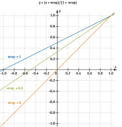
Figure 16-1 Graph of the Wrap Lighting Function

 float diffuse = max(0, dot(L, N)); float wrap_diffuse = max(0, (dot(L, N) + wrap) / (1 + wrap));

To compute this efficiently in a fragment program, the function can be encoded in a texture, which is indexed by the dot product between the light vector and the normal. This texture can also be created to include a slight color shift toward red when the lighting approaches zero. This is a cheap way to simulate scattering for skin shaders. The same texture can also include the power function for specular lighting in the alpha channel. The FX code in Listing 16-1 demonstrates how to use this technique. See Figure 16-2 for examples.

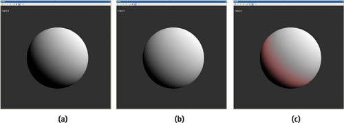
Figure 16-2 Applying Wrap Lighting to Spheres

Example 16-1. Excerpt from the Skin Shader Effect Incorporating Wrap Lighting

 // Generate 2D lookup table for skin shading 
   float4 GenerateSkinLUT(float2 P : POSITION) : COLOR {   float wrap = 0.2;   float scatterWidth = 0.3;   float4 scatterColor = float4(0.15, 0.0, 0.0, 1.0);   float shininess = 40.0; 
  float NdotL = P.x * 2 - 1;  // remap from [0, 1] to [-1, 1] 
    float NdotH = P.y * 2 - 1; 
  float NdotL_wrap = (NdotL + wrap) / (1 + wrap); // wrap lighting     float diffuse = max(NdotL_wrap, 0.0); 
  // add color tint at transition from light to dark     float scatter = smoothstep(0.0, scatterWidth, NdotL_wrap) *                     smoothstep(scatterWidth * 2.0, scatterWidth,                                NdotL_wrap); 
  float specular = pow(NdotH, shininess);   if (NdotL_wrap <= 0) specular = 0;   float4 C;   C.rgb = diffuse + scatter * scatterColor;   C.a = specular;   return C; } 
// Shade skin using lookup table 
   half3 ShadeSkin(sampler2D skinLUT,                 half3 N,                 half3 L,                 half3 H,                 half3 diffuseColor,                 half3 specularColor) : COLOR {   half2 s;   s.x = dot(N, L);   s.y = dot(N, H);   half4 light = tex2D(skinLUT, s * 0.5 + 0.5);   return diffuseColor * light.rgb + specularColor * light.a; }

16.3 Simulating Absorption Using Depth Maps

One of the most important factors in simulating very translucent materials is absorption. The farther through the material light travels, the more it is scattered and absorbed. To simulate this effect, we need a measure of the distance light has traveled through the material.

One method of estimating this distance is to use depth maps (Hery 2002). This technique is very similar to shadow mapping, and it is practical for real-time rendering. In the first pass, we render the scene from the point of view of the light, storing the distance from the light to a texture. This image is then projected back onto the scene using standard projective texture mapping. In the rendering pass, given a point to be shaded, we can look up into this texture to obtain the distance from the light at the point the ray entered the surface (d_i ). By subtracting this value from the distance from the light to the point at which the ray exited the surface (d_o ), we obtain an estimate of the distance the light has traveled through the object (s). See Figure 16-3.

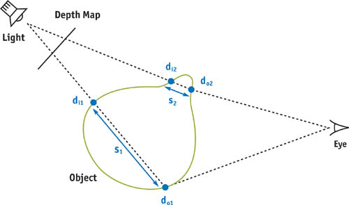
Figure 16-3 Calculating the Distance Light Has Traveled Through an Object Using a Depth Map

The obvious problem with this technique is that it works only with convex objects: holes within the object are not accounted for correctly. In practice, this is not a big issue, but it may be possible to get around the problem using depth peeling, which removes layers of the object one by one (Everitt 2003).

You might be thinking that for static objects, it would be possible to paint or precalculate a map that represents the approximate thickness of the surface at each point. The advantage of using depth maps is they take into account the direction of the incoming light, and they also work for animating models (assuming that you regenerate the depth map each frame).

The programs in Listings 16-2 and 16-3 demonstrate how to render distance from the light to a texture. They assume the modelView and modelViewProj matrices have been set up by the application for the light view.

Example 16-2. The Vertex Program for the Depth Pass

 struct a2v {   float4 pos    : POSITION;   float3 normal : NORMAL; }; struct v2f {   float4 hpos : POSITION;   float  dist : TEXCOORD0; // distance from light }; 
v2f main(a2v IN,          uniform float4x4 modelViewProj,          uniform float4x4 modelView,          uniform float    grow) {   v2f OUT;   float4 P = IN.pos;   P.xyz += IN.normal * grow;  // scale vertex along normal   OUT.hpos = mul(modelViewProj, P);   OUT.dist = length(mul(modelView, IN.pos));   return OUT; }

Example 16-3. The Fragment Program for the Depth Pass

 float4 main(float dist : TEX0) : COLOR {   return dist;  // return distance }

The fragment program extract in Listing 16-4 shows how to look up in the light distance texture to calculate depth. For flexibility, this code does the projection in the fragment program, but if you are taking only a few samples, it will be more efficient to calculate these transformations in the vertex program.

Example 16-4. The Fragment Program Function for Calculating Penetration Depth Using Depth Map

 // Given a point in object space, lookup into depth textures 
   // returns depth 
   float trace(float3 P,             uniform float4x4  lightTexMatrix, // to light texture space     uniform float4x4  lightMatrix,    // to light space     uniform sampler2D lightDepthTex,             ) {   // transform point into light texture space     float4 texCoord = mul(lightTexMatrix, float4(P, 1.0)); 
  // get distance from light at entry point     float d_i = tex2Dproj(lightDepthTex, texCoord.xyw); 
  // transform position to light space     float4 Plight = mul(lightMatrix, float4(P, 1.0)); 
  // distance of this pixel from light (exit)     float d_o = length(Plight); 
  // calculate depth     float s = d_o - d_i;   return s; }

Once we have a measure of the distance the light has traveled through the material, there are several ways we can use it. One simple way is to use it to index directly into an artist-created 1D texture that maps distance to color. The color should fall off exponentially with distance. By changing this color map, and combining the effect with other, more traditional lighting models, we can produce images of different materials, such as marble or jade.

 float si = trace(IN.objCoord, lightTexMatrix, lightMatrix,                  lightDepthTex); return tex1D(scatterTex, si);

Alternatively, we can evaluate the exponential function directly:

 return exp(-si * sigma_t) * lightColor;

The problem with this technique is that it does not simulate the way light is diffused as it passes through the object. When the light is behind the object, you will often clearly see features from the back side of the object showing through on the front. The solution to this is to take multiple samples at different points on the surface or to use a different diffusion approximation, as discussed in the next section.

16.3.1 Implementation Details

On GeForce FX hardware, when reading from a depth texture, only the most significant eight bits of the depth value are available. This is not sufficient precision. Instead, we can either use floating-point textures or use the pack and unpack instructions from the NVIDIA fragment program extension to store a 32-bit float value in a regular eight-bit RGBA texture. Floating-point textures do not currently support filtering, so block artifacts will sometimes be visible where the projected texture is magnified. If necessary, bilinear filtering can be performed in the shader, at some performance cost.

Another problem with projected depth maps is that artifacts often appear around the edges of the projection. These are similar to the self-shadowing artifacts seen with shadow mapping. They result mainly from the limited resolution of the texture map, which causes pixels from the background to be projected onto the edges of the object. The sample code avoids this problem by slightly scaling the object along the vertex normal during the depth-map pass.

For more accurate simulations, we may also need to know the normal, and potentially the surface color, at the point at which the light entered the object. We can achieve this by rendering additional passes that render the extra information to textures. We can look up in these textures in a similar way to the depth texture. On systems that support multiple render targets, it may be possible to collapse the depth, normal, and other passes into a single pass that outputs multiple values. See Figure 16-4.

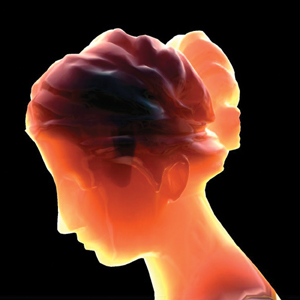
Figure 16-4 Using a Depth Map to Approximate Scattering

16.3.2 More Sophisticated Scattering Models

More sophisticated models attempt to accurately simulate the cumulative effects of scattering within the medium.

One model is the single scattering approximation, which assumes that light bounces only once within the material. By stepping along the refracted ray into the material, one can estimate how many photons would be scattered toward the camera. Phase functions are used to describe the distribution of directions in which light is scattered when it hits a particle. It is also important to take into account the Fresnel effect at the entry and exit points.

Another model, the diffusion approximation, simulates the effect of multiple scattering for highly scattering media, such as skin.

Unfortunately, these techniques are beyond the scope of this chapter.

Christophe Hery's chapter from the SIGGRAPH 2003 RenderMan course (Hery 2003) goes into the details of single and diffusion scattering for skin shaders.

16.4 Texture-Space Diffusion

As we noted earlier, one of the most obvious visual signs of subsurface scattering is a general blurring of the effects of lighting. In fact, 3D artists often emulate this phenomenon in screen space by performing Gaussian blurs of their renders in Adobe Photoshop and then adding a small amount of the blurred image back on top of the original. This "glow" technique softens the lighting and makes the images look less computer-generated.

It is possible to simulate diffusion in texture space (Borshukov and Lewis 2003). We can unwrap the mesh of the object with a vertex program that uses the UV texture coordinates as the screen position of the vertex. The program simply remaps the [0, 1] range of the texture coordinates to the [–1, 1] range of normalized device coordinates. We have to be careful that the object has a good UV mapping; that is, each point on the texture must map to only one point of the object, with no overlaps. By lighting this unwrapped mesh in the normal way, we obtain a 2D image representing the lighting of the object. We can then process this image and reapply it to the 3D model like a normal texture.

The vertex program in Listing 16-5 demonstrates how to render a model in UV space and perform diffuse lighting.

This technique is useful for other applications, because it decouples the shading complexity from the screen resolution: shading is performed only for each texel in the texture map, rather than for every pixel on the object. Many operations, such as convolutions, can be performed much more efficiently in image space than on a 3D surface. If the UV parameterization of the surface is relatively uniform, this is not a bad approximation, because points that are close in world space will map to points that are also close in texture space.

To simulate light diffusion in image space, we can simply blur the light map texture. We can take advantage of all the usual GPU image-processing tricks, such as using separable filters and exploiting bilinear filtering hardware. Rendering the lighting to a relatively low-resolution texture already provides a certain amount of blurring. Figure 16-5 shows an unwrapped head mesh and the results of blurring the light map texture.

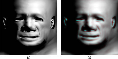
Figure 16-5 Unwrapped Head Mesh

Example 16-5. A Vertex Program to Unwrap a Model and Perform Diffuse Lighting

 struct a2v {   float4 pos     : POSITION;   float3 normal  : NORMAL;   float2 texture : TEXCOORD0; }; 
struct v2f {   float4 hpos     : POSITION;   float2 texcoord : TEXCOORD0;   float4 col      : COLOR0; }; 
v2f main(a2v IN,          uniform float4x4 lightMatrix) {   v2f OUT; 
  // convert texture coordinates to NDC position [-1, 1]   OUT.hpos.xy = IN.texture * 2 - 1;   OUT.hpos.z = 0.0;   OUT.hpos.w = 1.0; 
  // diffuse lighting     float3 N = normalize(mul((float3x3) lightMatrix, IN.normal));   float3 L = normalize(-mul(lightMatrix, IN.pos).xyz);   float diffuse = max(dot(N, L), 0);   OUT.col = diffuse; 
  OUT.texcoord = IN.texture;   return OUT; }

A diffuse color map can also be included in the light map texture; then details from the color map will also be diffused. If shadows are included in the texture, the blurring process will result in soft shadows.

To simulate the fact that absorption and scattering are wavelength dependent, we can alter the filter weights separately for each color channel. The sample shader, shown in Listings 16-6 and 16-7, attempts to simulate skin. It takes seven texture samples with Gaussian weights. The width of the filter is greater for the red channel than for the green and blue channels, so that the red is diffused more than the other channels. The vertex program in Listing 16-6 calculates the sample positions for a blur in the x direction; the program for the y direction is almost identical. The samples are spaced two texels apart to take advantage of the bilinear filtering capability of the hardware.

Example 16-6. The Vertex Program for Diffusion Blur

 v2f main(float2 tex : TEXCOORD0) {   v2f OUT;   // 7 samples, 2 texel spacing   OUT.tex0 = tex + float2(-5.5, 0);   OUT.tex1 = tex + float2(-3.5, 0);   OUT.tex2 = tex + float2(-1.5, 0);   OUT.tex3 = tex + float2(0, 0);   OUT.tex4 = tex + float2(1.5, 0);   OUT.tex5 = tex + float2(3.5, 0);   OUT.tex6 = tex + float2(5.5, 0);   return OUT; }

Example 16-7. The Fragment Program for Diffusion Blur

 half4 main(v2fConnector v2f,            uniform sampler2D lightTex            ) : COLOR {   // weights to blur red channel more than green and blue     const float4 weight[7] = {     { 0.006, 0.0,  0.0,  0.0 },     { 0.061, 0.0,  0.0,  0.0 },     { 0.242, 0.25, 0.25, 0.0 },     { 0.383, 0.5,  0.5,  0.0 },     { 0.242, 0.25, 0.20, 0.0 },     { 0.061, 0.0,  0.0,  0.0 },     { 0.006, 0.0,  0.0,  0.0 },   }; 
  half4 a;   a  = tex2D(lightTex, v2f.tex0) * weight[0];   a += tex2D(lightTex, v2f.tex1) * weight[1];   a += tex2D(lightTex, v2f.tex2) * weight[2];   a += tex2D(lightTex, v2f.tex3) * weight[3];   a += tex2D(lightTex, v2f.tex4) * weight[4];   a += tex2D(lightTex, v2f.tex5) * weight[5];   a += tex2D(lightTex, v2f.tex6) * weight[6];   return a; }

To achieve a wider blur, you can either apply the blur shader several times or write a shader that takes more samples by calculating the sample positions in the fragment program. Figure 16-6 shows the blurred light map texture applied back onto the 3D head model.

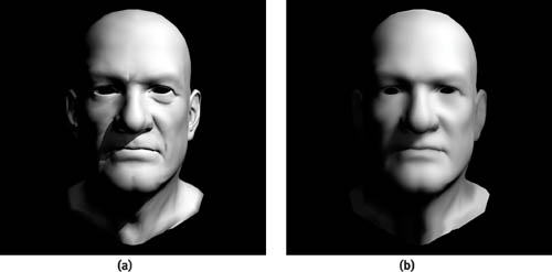
Figure 16-6 Texture-Space Diffusion on a Head Model

The final shader blends the diffused lighting texture with the original high-resolution color map to obtain the final effect, as shown in Figure 16-7.

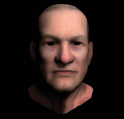
Figure 16-7 The Final Model, with Color Map

16.4.1 Possible Future Work

One possible extension to the depth map technique would be to render additional depth passes to account for denser objects within the object, such as bones within a body. The problem is that we are trying to account for volumetric effects using a surface-based representation. Volume rendering does not have this restriction, and it can produce much more accurate renderings of objects whose density varies. For more on volume rendering, see Chapter 39 of this book, "Volume Rendering Techniques."

Another possible extension to this technique would be to provide several color maps, each representing the color of a different layer of skin. For example, you might provide one map for the surface color and another for the veins and capillaries underneath the skin.

Greg James (2003) describes a technique that handles arbitrary polygonal objects by first adding up the distances of all the back-facing surfaces and then subtracting the distances of all the front-facing surfaces. His application computes distances in screen space for volumetric fog effects, but it could be extended to more general situations.

An interesting area of future research is combining the depth-map and texture-space techniques to obtain the best of both worlds.

16.5 Conclusion

The effects of subsurface scattering are an important factor in producing convincing images of skin and other translucent materials. By using several different approximations, we have shown how to achieve much of the look of subsurface scattering today in real time. As graphics hardware becomes more powerful, increasingly accurate models of subsurface light transport will be possible.

We hope that the techniques described in this chapter will inspire you to improve the realism of real-time game characters. But remember, good shading can never help bad art!

16.6 References

Borshukov, George, and J. P. Lewis. 2003. "Realistic Human Face Rendering for 'The Matrix Reloaded.'" SIGGRAPH 2003. Available online at http://www.virtualcinematography.org/

Everitt, Cass. 2003. "Order-Independent Transparency." Available online at http://developer.nvidia.com/view.asp?IO=order_independent_transparency

Hery, Christophe. 2002. "On Shadow Buffers." Presentation available online at http://www.renderman.org/RMR/Examples/srt2002/PrmanUserGroup2002.ppt

Hery, Christophe. 2003. "Implementing a Skin BSSRDF." RenderMan course notes, SIGGRAPH 2003. Available online at http://www.renderman.org/RMR/Books/sig03.course09.pdf.gz

James, Greg. 2003. "Rendering Objects as Thick Volumes." In ShaderX2: Shader Programming Tips & Tricks With DirectX 9, edited by Wolfgang F. Engel. Wordware. More information available online at http://www.shaderx2.com

Jensen, Henrik Wann, Stephen R. Marschner, Marc Levoy, and Pat Hanrahan. 2001. "A Practical Model for Subsurface Light Transport." In Proceedings of SIGGRAPH 2001.

Nayar, S. K., and M. Oren. 1995. "Generalization of the Lambertian Model and Implications for Machine Vision." International Journal of Computer Vision 14, pp. 227–251.

Pharr, Matt. 2001. "Layer Media for Surface Shaders." Advanced RenderMan course notes, SIGGRAPH 2001. Available online at http://www.renderman.org/RMR/Books/sig01.course48.pdf.gz

Statue model courtesy of De Espona Infographica (http://www.deespona.com). Head model courtesy of Steven Giesler (http://www.stevengiesler.com).

Copyright

Many of the designations used by manufacturers and sellers to distinguish their products are claimed as trademarks. Where those designations appear in this book, and Addison-Wesley was aware of a trademark claim, the designations have been printed with initial capital letters or in all capitals.

The authors and publisher have taken care in the preparation of this book, but make no expressed or implied warranty of any kind and assume no responsibility for errors or omissions. No liability is assumed for incidental or consequential damages in connection with or arising out of the use of the information or programs contained herein.

The publisher offers discounts on this book when ordered in quantity for bulk purchases and special sales. For more information, please contact:

U.S. Corporate and Government Sales
(800) 382-3419
corpsales@pearsontechgroup.com

For sales outside of the U.S., please contact:

International Sales
international@pearsoned.com

Visit Addison-Wesley on the Web: www.awprofessional.com

Library of Congress Control Number: 2004100582

GeForce™ and NVIDIA Quadro^® are trademarks or registered trademarks of NVIDIA Corporation.
RenderMan^® is a registered trademark of Pixar Animation Studios.
"Shadow Map Antialiasing" © 2003 NVIDIA Corporation and Pixar Animation Studios.
"Cinematic Lighting" © 2003 Pixar Animation Studios.
Dawn images © 2002 NVIDIA Corporation. Vulcan images © 2003 NVIDIA Corporation.

All rights reserved. No part of this publication may be reproduced, stored in a retrieval system, or transmitted, in any form, or by any means, electronic, mechanical, photocopying, recording, or otherwise, without the prior consent of the publisher. Printed in the United States of America. Published simultaneously in Canada.

For information on obtaining permission for use of material from this work, please submit a written request to:

Pearson Education, Inc.
Rights and Contracts Department
One Lake Street
Upper Saddle River, NJ 07458

Text printed on recycled and acid-free paper.

5 6 7 8 9 10 QWT 09 08 07

5th Printing September 2007

Part II: Lighting and Shadows

Part III: Materials

Part IV: Image Processing

Part V: Performance and Practicalities

Part VI: Beyond Triangles

Preface