GPU Gems

GPU Gems is now available, right here, online. You can purchase a beautifully printed version of this book, and others in the series, at a 30% discount courtesy of InformIT and Addison-Wesley.

The CD content, including demos and content, is available on the web and for download.

Chapter 14. Perspective Shadow Maps: Care and Feeding

Simon Kozlov
SoftLab-NSK

14.1 Introduction

Shadow generation has always been a big problem in real-time 3D graphics. Determining whether a point is in shadow is not a trivial operation for modern GPUs, particularly because GPUs work in terms of rasterizing polygons instead of ray tracing.

Today's shadows should be completely dynamic. Almost every object in the scene should cast and receive shadows, there should be self-shadowing, and every object should have soft shadows. Only two algorithms can satisfy these requirements: shadow volumes (or stencil shadows) and shadow mapping.

The difference between the algorithms for shadow volumes and shadow mapping comes down to object space versus image space:

Object-space shadow algorithms, such as shadow volumes, work by creating a polygonal structure that represents the shadow occluders, which means that we always have pixel-accurate, but hard, shadows. This method cannot deal with objects that have no polygonal structure, such as alpha-test-modified geometry or displacement mapped geometry. Also, drawing shadow volumes requires a lot of fill rate, which makes it difficult to use them for every object in a dense scene, especially when there are multiple lights.
Image-space shadow algorithms deal with any object modification (if we can render an object, we'll have shadows), but they suffer from aliasing. Aliasing often occurs in large scenes with wide or omnidirectional light sources. The problem is that the projection transform used in shadow mapping changes the screen size of the shadow map texels so that texels near the camera become very large. As a result, we have to use enormous shadow maps (four times the screen resolution or larger) to achieve good quality. Still, shadow maps are much faster than shadow volumes in complex scenes.

Perspective shadow maps (PSMs), presented at SIGGRAPH 2002 by Stamminger and Drettakis (2002), try to eliminate aliasing in shadow maps by using them in post-projective space, where all nearby objects become larger than farther ones. Unfortunately, it's difficult to use the original algorithm because it works well only in certain cases.

The most significant problems of the presented PSM algorithm are these three:

To hold all potential shadow casters inside the virtual camera frustum, "virtual cameras" are used when the light source is behind the camera. This results in poor shadow quality.
The shadow quality depends heavily on the light position in camera space.
Biasing problems weren't discussed in the original paper. Bias is a problem with PSMs because the texel area is distributed in a nonuniform way, which means that bias cannot be a constant anymore and should depend on the texel position.

Each of these problems is discussed in the next section. This chapter focuses on directional lights (because they have bigger aliasing problems), but all the ideas and algorithms can easily be applied to other types of light source (details are provided, where appropriate). In addition, we discuss tricks for increasing the quality of the shadow map by filtering and blurring the picture.

In general, this chapter describes techniques and methods that can increase the effectiveness of using PSMs. However, most of these ideas still should be adapted to your particular needs.

14.2 Problems with the PSM Algorithm

14.2.1 Virtual Cameras

First, let's look at the essence of this problem. The usual projective transform moves objects behind the camera to the other side of the infinity plane in post-projective space. However, if the light source is behind the camera too, these objects are potential shadow casters and should be drawn into the shadow map.

In the perspective transform in Figure 14-1, the order of the points on the ray changes. The authors of the original PSM paper propose "virtually" sliding the view camera back to hold potential shadow casters in the viewing frustum, as shown in Figure 14-2, so that we can use PSMs the normal way.

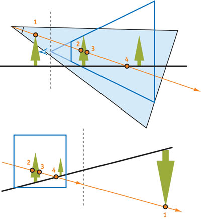
Figure 14-1 An Object Behind the Camera in Post-Projective Space

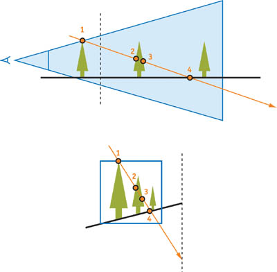
Figure 14-2 Using a Virtual Camera

Virtual Camera Issues

In practice, however, using the virtual camera leads to poor shadow quality. The "virtual" shift greatly decreases the resolution of the effective shadow map, so that objects near the real camera become smaller, and we end up with a lot of unused space in the shadow map. In addition, we may have to move the camera back significantly for large shadow-casting objects behind the camera. Figure 14-3 shows how dramatically the quality changes, even with a small shift.

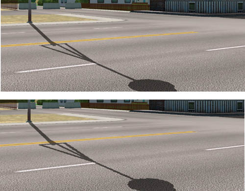
Figure 14-3 The Effect of the Virtual Shift on Shadow Quality

Another problem is minimizing the actual "slideback distance," which maximizes image quality. This requires us to analyze the scene, find potential shadow casters, and so on. Of course, we could use bounding volumes, scene hierarchical organizations, and similar techniques, but they would be a significant CPU hit. Moreover, we'll always have abrupt changes in shadow quality when an object stops being a potential shadow caster. In this case, the slideback distance instantly changes, causing the shadow quality to change suddenly as well.

A Solution for Virtual Camera Issues

We propose a solution to this virtual camera problem: Use a special projection transform for the light matrix. In fact, post-projective space allows some projection tricks that can't be done in the usual world space. It turns out that we can build a special projection matrix that can see "farther than infinity."

Let's look at a post-projective space formed by an original (nonvirtual) camera with a directional "inverse" light source and with objects behind the view camera, as shown in Figure 14-4.

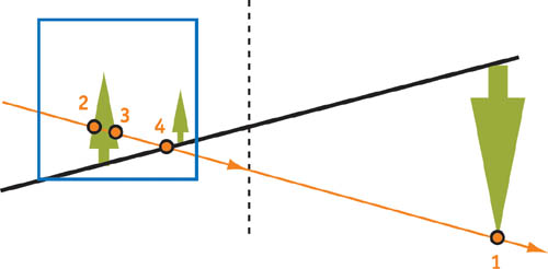
Figure 14-4 Post-Projective Space with an Inverse Light Source

A drawback to this solution is that the ray should (but doesn't) come out from the light source, catch point 1, go to minus infinity, then pass on to plus infinity and return to the light source, capturing information at points 2, 3, and 4. Fortunately, there is a projection matrix that matches this "impossible" ray, where we can set the near plane to a negative value and the far plane to a positive value. See Figure 14-5.

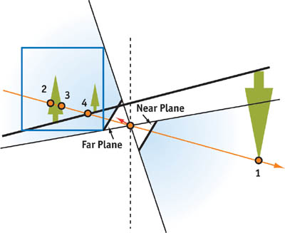
Figure 14-5 An Inverse Projection Matrix

In the simplest case,

where a is small enough to fit the entire unit cube. Then we build this inverse projection as the usual projection matrix, as shown here, where matrices are written in a row-major style:

So the formula for the resulting transformed z coordinates, which go into a shadow map, is:

Z _psm (-a) = 0 , and if we keep decreasing the z value to minus infinity, Z _psm tends to ½. The same Z _psm = ½ corresponds to plus infinity, and moving from plus infinity to the far plane increases Z _psm to 1 at the far plane. This is why the ray hits all points in the correct order and why there's no need to use "virtual slides" for creating post-projective space.

This trick works only in post-projective space because normally all points behind the infinity plane have w < 0, so they cannot be rasterized. But for another projection transformation caused by a light camera, these points are located behind the camera, so the w coordinate is inverted again and becomes positive.

By using this inverse projection matrix, we don't have to use virtual cameras. As a result, we get much better shadow quality without any CPU scene analysis and the associated artifacts.

The only drawback to the inverse projection matrix is that we need a better shadow map depth-value precision, because we use big z-value ranges. However, 24-bit fixed-point depth values are enough for reasonable cases.

Virtual cameras still could be useful, though, because the shadow quality depends on the location of the camera's near plane. The formula for post-projective z is:

As we can see, Q is very close to 1 and doesn't change significantly as long as Z _n is much smaller than Z _f , which is typical. That's why the near and far planes have to be changed significantly to affect the Q value, which usually is not possible. At the same time, near-plane values highly influence the post-projective space. For example, for Z _n = 1 meter (m), the first meter in the world space after the near plane occupies half the unit cube in post-projective space. In this respect, if we change Z _n to 2 m, we will effectively double the z-value resolution and increase the shadow quality. That means that we should maximize the Z _n value by any means.

The perfect method, proposed in the original PSM article, is to read back the depth buffer, scan through each pixel, and find the maximum possible Z _n for each frame. Unfortunately, this method is quite expensive: it requires reading back a large amount of video memory, causes an additional CPU/GPU stall, and doesn't work well with swizzled and hierarchical depth buffers. So we should use another (perhaps less accurate) method to find a suitable near-plane value for PSM rendering.

Such other methods for finding a suitable near-plane value for PSM rendering could include various methods of CPU scene analysis:

A method based on rough bounding-volume computations (briefly described later in "The Light Camera").
A collision-detection system to estimate the distance to the closest object.
Additional software scene rendering with low-polygon-count level-of-details, which could also be useful for occlusion culling.
Sophisticated analysis based on particular features of scene structure for the specific application. For example, when dealing with scenarios using a fixed camera path, you could precompute the near-plane values for every frame.

These methods try to increase the actual near-plane value, but we could also increase the value "virtually." The idea is the same as with the old virtual cameras, but with one difference. When sliding the camera back, we increase the near-plane value so that the near-plane quads of the original and virtual cameras remain on the same plane. See Figure 14-6.

Figure 14-6 Difference Between Virtual Cameras

When we slide the virtual camera back, we improve the z-values resolution. However, this makes the value distribution for x and y values worse for near objects, thus balancing shadow quality near and far from the camera. Because of the very irregular z-value distribution in post-projective space and the large influence of the near-plane value, this balance could not be achieved without this "virtual" slideback. The usual problem of shadows looking great near the camera but having poor quality on distant objects is the typical result of unbalanced shadow map texel area distribution.

14.2.2 The Light Camera

Another problem with PSMs is that the shadow quality relies on the relationship between the light and camera positions. With a vertical directional light, aliasing problems are completely removed, but when light is directed toward the camera and is close to head-on, there is significant shadow map aliasing.

We're trying to hold the entire unit cube in a single shadow map texture, so we have to make the light's field of view as large as necessary to fit the entire cube. This in turn means that the objects close to the near plane won't receive enough texture samples. See Figure 14-7.

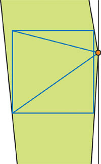
Figure 14-7 The Light Camera with a Low Light Angle

The closer the light source is to the unit cube, the poorer the quality. As we know,

so for large outdoor scenes that have Z _n = 1 and Z _f = 4000, Q = 1.0002, which means that the light source is extremely close to the unit cube. The Z_f /Z_n correlation is usually bigger than 50, which corresponds to Q = 1.02, which is close enough to create problems.

We'll always have problems fitting the entire unit cube into a single shadow map texture. Two solutions each tackle one part of the problem: Unit cube clipping targets the light camera only on the necessary part of the unit cube, and the cube map approach uses multiple textures to store depth information.

Unit Cube Clipping

This optimization relies on the fact that we need shadow map information only on actual objects, and the volume occupied by these objects is usually much smaller than the whole view frustum volume (especially close to the far plane). That's why if we tune the light camera to hold real objects only (not the entire unit cube), we'll receive better quality. Of course, we should tune the camera using a simplified scene structure, such as bounding volumes.

Cube clipping was mentioned in the original PSM article, but it took into account all objects in a scene, including shadow casters in the view frustum and potential shadow casters outside the frustum for constructing the virtual camera. Because we don't need virtual cameras anymore, we can focus the light camera on shadow receivers only, which is more efficient. See Figure 14-8. Still, we should choose near and far clip-plane values for the light camera in post-projective space to hold all shadow casters in the shadow map. But it doesn't influence shadow quality because it doesn't change the texel area distribution.

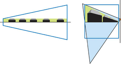
Figure 14-8 Focusing the Light Camera Based on the Bounding Volumes of Shadow Receivers

Because faraway parts of these bounding volumes contract greatly in post-projective space, the light camera's field of view doesn't become very large, even with light sources that are close to the rest of the scene.

In practice, we can use rough bounding volumes to retain sufficient quality—we just need to indicate generally which part of the scene we are interested in. In outdoor scenes, it's the approximate height of objects on the landscape; in indoor scenes, it's a bounding volume of the current room, and so on.

We'd like to formalize the algorithm of computing the light camera focused on shadow receivers in the scene after we build a set of bounding volumes roughly describing the scene. In fact, the light camera is given by position, direction, up vector, and projection parameters, most of which are predefined:

We can't change the position: it's a light position in post-projective space and nothing else.
In practice, the up vector doesn't change quality significantly, so we can choose anything reasonable.
Projection parameters are entirely defined by the view matrix.

So the most interesting thing is choosing the light camera direction based on bounding volumes. The proposed algorithm is this:

Compute the vertex list of constructive solid geometry operation, where B _i is the ith bounding volume, F is the frustum for every shadow caster bounding volume that we see in the current frame, and all these operations are performed in a view camera space. Then transform all these vertices into post-projective space. After this step, we have all the points that the light camera should "see." (By the way, we should find a good near-plane value based on these points, because reading back the depth buffer isn't a good solution.)
Find a light camera. As we already know, this means finding the best light camera direction, because all other parameters are easily computed for a given direction. We propose approximating the optimal direction by the axis of the minimal cone, centered in the light source and including all the points in the list. The algorithm that finds the optimal cone for a set of points works in linear time, and it is similar to an algorithm that finds the smallest bounding sphere for a set of points in linear time (Gartner 1999).

In this way, we could find an optimal light camera in linear time depending on the bounding volume number, which isn't very large because we need only rough information about the scene structure.

This algorithm is efficient for direct lights in large outdoor scenes. The shadow quality is almost independent of the light angle and slightly decreases if light is directed toward the camera. Figure 14-9 shows the difference between using unit cube clipping and not using it.

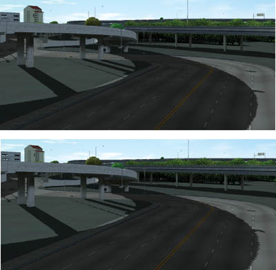
Figure 14-9 Unit Cube Clipping

Using Cube Maps

Though cube clipping is efficient in some cases, other times it's difficult to use. For example, we might have a densely filled unit cube (which is common), or we may not want to use bounding volumes at all. Plus, cube clipping does not work with point lights.

A more general method is to use a cube map texture for shadow mapping. Most light sources become point lights in post-projective space, and it's natural to use cube maps for shadow mapping with point light sources. But in post-projective space, things change slightly and we should use cube maps differently because we need to store information about the unit cube only.

The proposed solution is to use unit cube faces that are back facing, with respect to the light, as platforms for cube-map-face textures.

For a direct light source in post-projective space, the cube map looks like Figure 14-10.

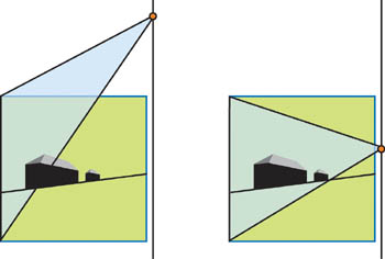
Figure 14-10 Using a Cube Map for Direct Lights

The number of used cube map faces (ranging from three to five) depends on the position of the light. We use the maximum number of faces when the light is close to the rest of the scene and directed toward the camera, so additional texture resources are necessary. For other types of light sources located outside the unit cube, the pictures will be similar.

For a point light located inside the unit cube, we should use all six cube map faces, but they're still focused on unit cube faces. See Figure 14-11.

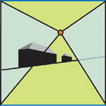
Figure 14-11 Using Cube Maps with a Point Light

We could say we form a "cube map with displaced center," which is similar to a normal cube map, but with a constant vector added to its texture coordinates. In other words, texture coordinates for cube maps are vertex positions in post-projective space shifted by the light source position:

Texture coordinates = vertex position - light position

By choosing unit cube faces as the cube map platform, we distribute the texture area proportionally to the screen size and ensure that shadow quality doesn't depend on the light and camera positions. In fact, texel size in post-projective space is in a guaranteed range, so its projection on the screen depends only on the plane it's projected onto. This projection doesn't stretch texels much, so the texel size on the screen is within guaranteed bounds also.

Because the vertex and pixel shaders are relatively short when rendering the shadow map, what matters is the pure fill rate for the back buffer and the depth shadow map buffer. So there's almost no difference between drawing a single shadow map and drawing a cube map with the same total texture size (with good occlusion culling, though). The cube map approach has better quality with the same total texture size as a single texture. The difference is the cost of the render target switch and the additional instructions to compute cube map texture coordinates in the vertex and pixel shaders.

Let's see how to compute these texture coordinates. First, consider the picture shown in Figure 14-12. The blue square is our unit cube, P is the light source point, and V is the point for which we're generating texture coordinates. We render all six cube map faces in separate passes for the shadow map; the near plane for each pass is shown in green. They're forming another small cube, so Z ₁ = Z _n /Z _f is constant for every pass.

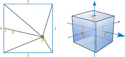
Figure 14-12 A Detailed Cube Map View in Post-Projective Space

Now we should compute texture coordinates and depth values to compare for the point V. This just means that we should move this point in the (V - P ) direction until we intersect the cube. Consider d ₁, d ₂, d ₃, d ₄, d ₅, and d ₆ (see the face numbers in Figure 14-12) as the distances from P to each cube map face.

The point on the cube we are looking for (which is also the cube map texture coordinate) is:

Compare the value in the texture against the result of the projective transform of the a value. Because we already divided it by the corresponding d value, thus effectively making Z _f = 1 and Z _n = Z ₁, all we have to do is apply that projective transform. Note that in the case of the inverse camera projection from Section 14.2.1, Z _n = -Z ₁, Z _f = Z ₁.

(All these calculations are made in OpenGL-like coordinates, where the unit cube is actually a unit cube. In Direct3D, the unit cube is half the size, because the z coordinate is in the [0..1] range.)

Listing 14-1 is an example of how the shader code might look.

Example 14-1. Shader Code for Computing Cube Map Texture Coordinates

 // c[d1] = 1/d1, 1/d2, 1/d3, 0 
// c[d2] = -1/d4, -1/d5, -1/d6, 0 
// c[z] = Q, -Q * Zn, 0, 0 
// c[P] = P 
// r[V] = V 
// cbmcoord - output cube map texture coordinates 
// depth - depth to compare with shadow map values 
 //Per-vertex level 
sub r[VP], r[V], c[P] mul r1, r[VP], c[d1] mul r2, r[VP], c[d2] 
//Per-pixel level 
max r3, r1, r2 max r3.x, r3.x, r3.y max r3.x, r3.x, r3.z rcp r3.w, r3.x mad cbmcoord, r[VP], r3.w, c[P] 
rcp r3.x, r3.w mad depth, r3.x, c[z].x, c[z].y

Because depth textures cannot be cube maps, we could use color textures, packing depth values into the color channels. There are many ways to do this and many implementation-dependent tricks, but their description is out of the scope of this chapter.

Another possibility is to emulate this cube map approach with multitexturing, in which every cube map face becomes an independent texture (depth textures are great in this case). We form several texture coordinate sets in the vertex shader and multiply by the shadow results in the pixel shader. The tricky part is to manage these textures over the objects in the scene, because every object rarely needs all six faces.

14.2.3 Biasing

As we stated earlier, the constant bias that is typically used in uniform shadow maps cannot be used with PSMs because the z values and the texel area distributions vary greatly with different light positions and points in the scene.

If you plan to use depth textures, try z slope–scaled bias for biasing. It's often enough to fix the artifacts, especially when very distant objects don't fall within the camera. However, some cards do not support depth textures (in DirectX, depth textures are supported only by NVIDIA cards), and depth textures can't be a cube map. In these cases, you need a different, more general algorithm for calculating bias. Another difficulty is that it's hard to emulate and tweak z slope–scaled bias because it requires additional data—such as the vertex coordinates of the current triangle—passed into the pixel shader, plus some calculations, which isn't robust at all.

Anyway, let's see why we can't use constant bias anymore. Consider these two cases: the light source is near the unit cube, and the light source is far from the unit cube. See Figure 14-13.

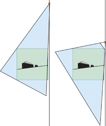
Figure 14-13 Light Close to and Far from the Unit Cube

The problem is that the Z _f /Z _n correlation, which determines the z-value distribution into a shadow map, varies a lot in these two cases. So the constant bias would mean a totally different actual bias in world and post-projective space: The constant bias tuned to the first light position won't be correct for the second light, and vice versa. Meanwhile, Z _f /Z _n changes a lot, because the light source could be close to the unit cube and could be distant (even at infinity), depending on the relative positions of the light and the camera in world space.

Even with a fixed light source position, sometimes we cannot find a suitable constant for the bias. The bias should depend on the point position—because the projective transform enlarges the near objects and shrinks the far ones—so the bias should be smaller near the camera and bigger for distant objects. Figure 14-14 shows the typical artifacts of using a constant bias in this situation.

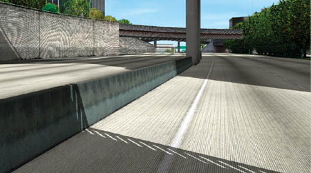
Figure 14-14 Artifacts with Constant Bias

In short, the proposed solution is to use biasing in world space (and not to analyze the results of the double-projection matrix) and then transform this world-space bias in post-projective space. The computed value depends on the double projection, and it's correct for any light and camera position. These operations could be done easily in a vertex shader. Furthermore, this world-space bias value should be scaled by texel size in world space to deal with artifacts caused by the distribution of nonuniform texel areas.

P_biased = (P _orig + L(a + bL_texel ))M,

where P _orig is the original point position, L is the light vector direction in world space, L_texel is the texel size in world space, M is the final shadow map matrix, and a and b are bias coefficients.

The texel size in world space could be approximately computed with simple matrix calculations. First, transform the point into shadow map space, and then shift this point by the texel size without changing depth. Next, transform it back into world space and square the length of the difference between this point and the original one. This gives us L_texel :

and S _x and S _y are shadow map resolutions.

Obviously, we can build a single matrix that performs all the transformations (except multiplying the coordinates, of course):

where M' includes transforming, shifting, transforming back, and subtracting.

This turns out to be a rather empirical solution, but it should still be tweaked for your particular needs. See Figure 14-15.

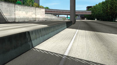
Figure 14-15 Bias Calculated in the Vertex Shader

The vertex shader code that performs these calculations might look like Listing 14-2.

Example 14-2. Calculating Bias in a Vertex Shader

 def c0, a, b, 0 ,0 
// Calculating Ltexel 
dp4 r1.x, v0, c[LtexelMatrix_0] dp4 r1.y, v0, c[LtexelMatrix_1] dp4 r1.z, v0, c[LtexelMatrix_2] dp4 r1.w, v0, c[LtexelMatrix_3] 
// Transforming homogeneous coordinates 
// (in fact, we often can skip this step) 
rcp r1.w, r1.w mul r1.xy, r1.w, r1.xy 
// Now r1.x is an Ltexel 
mad r1.x, r1.x, c0.x, c0.y 
dp3 r1.x, r1, r1 
// Move vertex in world space 
mad r1, v0, c[Lightdir], r1.x 
// Transform vertex into post-projective space 
// (we need z and w only) 
dp4 r[out].z, r1, c[M_2] dp4 r[out].w, r1, c[M_3]

The r[out] register holds the result of the biasing: the depth value, and the corresponding w, that should be interpolated across the triangle. Note that this interpolation should be separate from the interpolation of texture coordinates (x, y, and the corresponding w), because these w coordinates are different. This biased value could be used when comparing with the shadow map value, or during the actual shadow map rendering (the shadow map holds biased values).

14.3 Tricks for Better Shadow Maps

The advantage of shadow mapping over shadow volumes is the potential to create a color gradient between "shadowed" and "nonshadowed" samples, thus simulating soft shadows. This shadow "softness" doesn't depend on distance from the occluder, light source size, and so on, but it still works in world space. Blurring stencil shadows, on the other hand, is more difficult, although Assarsson et al. (2003) make significant progress.

This section covers methods of filtering and blurring shadow maps to create a fake shadow softness that has a constant range of blurring but still looks good.

14.3.1 Filtering

Most methods of shadow map filtering are based on the percentage-closer filtering (PCF) principle. The only difference among the methods is how the hardware lets us use it. NVIDIA depth textures perform PCF after comparison with the depth value; on other hardware, we have to take several samples from the nearest texels and average their results (for true PCF). In general, the depth texture filtering is more efficient than the manual PCF technique with four samples. (PCF needs about eight samples to produce comparable quality.) In addition, using depth texture filtering doesn't forbid PCF, so we can take several filtered samples to further increase shadow quality.

Using PCF with PSMs is no different from using it with standard shadow maps: samples from neighboring texels are used for filtering. On the GPU, this is achieved by shifting texture coordinates one texel in each direction. For a more detailed discussion of PCF, see Chapter 11, "Shadow Map Antialiasing."

The shader pseudocode for PCF with four samples looks like Listings 14-3 and 14-4.

These tricks improve shadow quality, but they do not hide serious aliasing problems. For example, if many screen pixels map to one shadow map texel, large stair-stepping artifacts will be visible, even if they are somewhat blurred. Figure 14-16 shows an aliased shadow without any filtering, and Figure 14-17 shows how PCF helps improve shadow quality but cannot completely remove aliasing artifacts.

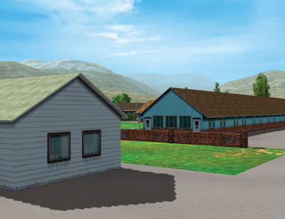
Figure 14-16 Strong Aliasing

Figure 14-17 Filtered Aliasing

Example 14-3. Vertex Shader Pseudocode for PCF

 def c0, sample1x, sample1Y, 0, 0 def c1, sample2x, sample2Y, 0, 0 def c2, sample3x, sample3Y, 0, 0 def c3, sample4x, sample4Y, 0, 0 // The simplest case: 
// def c0, 1 / shadowmapsizeX, 1 / shadowmapsizeY, 0, 0 
// def c1, -1 / shadowmapsizeX, -1 / shadowmapsizeY, 0, 0 
// def c2, -1 / shadowmapsizeX, 1/ shadowmapsizeY, 0, 0 
// def c3, 1 / shadowmapsizeX, -1 / shadowmapsizeY, 0, 0 
. . . 
// Point - vertex position in light space 
mad oT0, point.w, c0, point mad oT1, point.w, c1, point mad oT2, point.w, c2, point mad oT3, point.w, c3, point

Example 14-4. Pixel Shader Pseudocode for PCF

 def c0, 0.25, 0.25, 0.25, 0.25 tex t0 tex t1 tex t2 tex t3 
. . . 
// After depth comparison 
mul r0, t0, c0 mad r0, t1, c0, r0 mad r0, t2, c0, r0 mad r0, t3, c0, r0

14.3.2 Blurring

As we know from projective shadows, the best blurring results often come from rendering to a smaller resolution texture with a pixel shader blur, then feeding this resulting texture back through the blur pixel shader several times (known as ping-pong rendering). Shadow mapping and projective shadows are similar techniques, so why can't we use this method? The answer: because the shadow map isn't a black-and-white picture; it's a collection of depth values, and "blurring a depth map" doesn't make sense.

In fact, the proposal is to use the color part of the shadow map render (which comes almost for free) as projective texture for some objects. For example, assume that we have an outdoor landscape scene and we want a high-quality blurred shadow on the ground because ground shadows are the most noticeable.

Before rendering the depth shadow map, clear the color buffer with 1. During the render, draw 0 into the color buffer for every object except the landscape; for the landscape, draw 1 in color. After the whole shadow map renders, we'll have 1 where the landscape is nonshadowed and 0 where it's shadowed. See Figure 14-18.

Figure 14-18 The Original Color Part for a Small Test Scene
Blur the picture (the one in Figure 14-18) severely, using multiple passes with a simple blur pixel shader. For example, using a simple two-pass Gaussian blur gives good results. (You might want to adjust the blurring radius for distant objects.) After this step, we'll have a high-quality blurred texture, as shown in Figure 14-19.

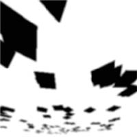
Figure 14-19 The Blurred Color Part for a Small Test Scene
While rendering the scene with shadows, render the landscape with the blurred texture instead of the shadow map, and render all other objects with the depth part of the shadow map. See Figure 14-20.

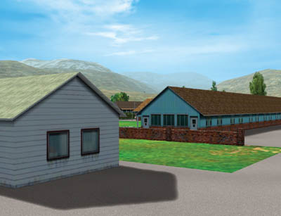
Figure 14-20 Applying Blurring to a Real Scene

The difference in quality is dramatic.

Of course, we can use this method not only with landscapes, but also with any object that does not need self-shadowing (such as floors, walls, ground planes, and so on). Fortunately, in these areas shadows are most noticeable and aliasing problems are most evident. Because we have several color channels, we can blur shadows on several objects at the same time:

Using depth textures, the color buffer is completely free, so we can use all four channels for four objects.
For floating-point textures, one channel stores depth information, so we have three channels for blurring.
For fixed-point textures, depth is usually stored in the red and green channels, so we have only two free channels.

This way we'll have nice blurred shadows on the ground, floor, walls, and so on while retaining all other shadows (blurred with PCF) on other objects (with proper self-shadowing).

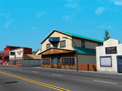
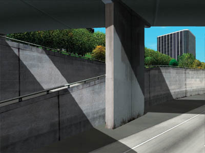
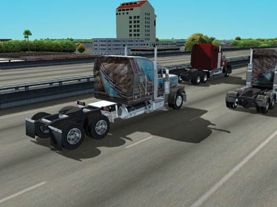
14.4 Results

The screenshots in Figures 14-21, 14-22, 14-23, and 14-24 were captured on the NVIDIA GeForce4 Ti 4600 in 1600x1200 screen resolution, with 100,000 to 500,000 visible polygons. All objects receive and cast shadows with real-time frame rates (more than 30).

14.5 References

Assarsson, U., M. Dougherty, M. Mounier, and T. Akenine-Möller. 2003. "An Optimized Soft Shadow Volume Algorithm with Real-Time Performance." In Proceedings of the SIGGRAPH/Eurographics Workshop on Graphics Hardware 2003.

Gartner, Bernd. 1999. "Smallest Enclosing Balls: Fast and Robust in C++." Web page. http://www.inf.ethz.ch/personal/gaertner/texts/own_work/esa99_final.pdf

Stamminger, Marc, and George Drettakis. 2002. "Perspective Shadow Maps." In Proceedings of ACM SIGGRAPH 2002.

The author would like to thank Peter Popov for his many helpful and productive discussions.

Copyright

Many of the designations used by manufacturers and sellers to distinguish their products are claimed as trademarks. Where those designations appear in this book, and Addison-Wesley was aware of a trademark claim, the designations have been printed with initial capital letters or in all capitals.

The authors and publisher have taken care in the preparation of this book, but make no expressed or implied warranty of any kind and assume no responsibility for errors or omissions. No liability is assumed for incidental or consequential damages in connection with or arising out of the use of the information or programs contained herein.

The publisher offers discounts on this book when ordered in quantity for bulk purchases and special sales. For more information, please contact:

U.S. Corporate and Government Sales
(800) 382-3419
corpsales@pearsontechgroup.com

For sales outside of the U.S., please contact:

International Sales
international@pearsoned.com

Visit Addison-Wesley on the Web: www.awprofessional.com

Library of Congress Control Number: 2004100582

GeForce™ and NVIDIA Quadro^® are trademarks or registered trademarks of NVIDIA Corporation.
RenderMan^® is a registered trademark of Pixar Animation Studios.
"Shadow Map Antialiasing" © 2003 NVIDIA Corporation and Pixar Animation Studios.
"Cinematic Lighting" © 2003 Pixar Animation Studios.
Dawn images © 2002 NVIDIA Corporation. Vulcan images © 2003 NVIDIA Corporation.

All rights reserved. No part of this publication may be reproduced, stored in a retrieval system, or transmitted, in any form, or by any means, electronic, mechanical, photocopying, recording, or otherwise, without the prior consent of the publisher. Printed in the United States of America. Published simultaneously in Canada.

For information on obtaining permission for use of material from this work, please submit a written request to:

Pearson Education, Inc.
Rights and Contracts Department
One Lake Street
Upper Saddle River, NJ 07458

Text printed on recycled and acid-free paper.

5 6 7 8 9 10 QWT 09 08 07

5th Printing September 2007

Part II: Lighting and Shadows

Part III: Materials

Part IV: Image Processing

Part V: Performance and Practicalities

Part VI: Beyond Triangles

Preface