
GPU Gems
GPU Gems is now available, right here, online. You can purchase a beautifully printed version of this book, and others in the series, at a 30% discount courtesy of InformIT and Addison-Wesley.
The CD content, including demos and content, is available on the web and for download.
Chapter 1. Effective Water Simulation from Physical Models
Mark Finch
Cyan Worlds
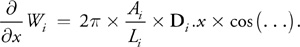
This chapter describes a system for simulating and rendering large bodies of water on the GPU. The system combines geometric undulations of a base mesh with generation of a dynamic normal map. The system has proven suitable for real-time game scenarios, having been used extensively in Cyan Worlds' Uru: Ages Beyond Myst, as shown in Figure 1-1.
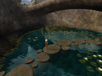
Figure 1-1 Tranquil Pond
1.1 Goals and Scope
Real-time rendering techniques have been migrating from the offline-rendering world over the last few years. Fast Fourier Transform (FFT) techniques, as outlined in Tessendorf 2001, produce incredible realism for sufficiently large sampling grids, and moderate-size grids may be processed in real time on consumer-level PCs. Voxel-based solutions to simplified forms of the Navier-Stokes equations are also viable (Yann 2003). Although we have not yet reached the point of cutting-edge, offline fluid simulations, as in Enright et al. 2002, the gap is closing. By the time this chapter is published, FFT libraries will likely be available for vertex and pixel shaders, but as of this writing, even real-time versions of these techniques are limited to implementation on the CPU.
At the same time, water simulation models simple enough to run on the GPU have been evolving upward as well. Isidoro et al. 2002 describes summing four sine waves in a vertex shader to compute surface height and orientation. Laeuchli 2002 presents a shader calculating surface height using three Gerstner waves.
We start with summing simple sine functions, then progress to slightly more complicated functions, as appropriate. We also extend the technique into the realm of pixel shaders, using a sum of periodic wave functions to create a dynamic tiling bump map to capture the finer details of the water surface.
This chapter focuses on explaining the physical significance of the system parameters, showing that approximating a water surface with a sum of sine waves is not as ad hoc as often presented. We pay special attention to the math that takes us from the underlying model to the actual implementation; the math is key to extending the implementation.
This system is designed for bodies of water ranging from a small pond to the ocean as viewed from a cove or island. Although not a rigorous physical simulation, it does deliver convincing, flexible, and dynamic renderings of water. Because the simulation runs entirely on the GPU, it entails no struggle over CPU usage with either artificial intelligence (AI) or physics processes. Because the system parameters do have a physical basis, they are easier to script than if they were found by trial and error. Making the system as a whole dynamic—in addition to its component waves—adds an extra level of life.
1.2 The Sum of Sines Approximation
We run two surface simulations: one for the geometric undulation of the surface mesh, and one for the ripples in the normal map on that mesh. Both simulations are essentially the same. The height of the water surface is represented by the sum of simple periodic waves. We start with summing sine functions and move to more interesting wave shapes as we go.
The sum of sines gives a continuous function describing the height and surface orientation of the water at all points. In processing vertices, we sample that function based on the horizontal position of each vertex, conforming the mesh to the limits of its tessellation to the continuous water surface. Below the resolution of the geometry, we continue the technique into texture space. We generate a normal map for the surface by sampling the normals of a sum of sines approximation through simple pixel shader operations in rendering to a render target texture. Rendering our normal map for each frame allows our limited set of sine waves to move independently, greatly enhancing the realism of the rendering.
In fact, the fine waves in our water texture dominate the realism of our simulation. The geometric undulations of our wave surface provide a subtler framework on which to present that texture. As such, we have different criteria for selecting geometric versus texture waves.
1.2.1 Selecting the Waves
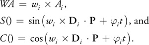
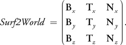
We need a set of parameters to define each wave. As shown in Figure 1-2, the parameters are:
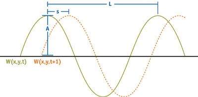
Figure 1-2 The Parameters of a Single Wave Function
- Wavelength (L): the crest-to-crest distance between waves in world space. Wavelength L relates to frequency w as w = 2/L.
- Amplitude (A): the height from the water plane to the wave crest.
- Speed (S): the distance the crest moves forward per second. It is convenient to express speed as phase-constant
 , where = S x 2/L.
 - Direction (D ): the horizontal vector perpendicular to the wave front along which the crest travels.
Then the state of each wave as a function of horizontal position (x, y) and time (t) is defined as:

And the total surface is:

over all waves i.
To provide variation in the dynamics of the scene, we will randomly generate these wave parameters within constraints. Over time, we will continuously fade one wave out and then fade it back in with a different set of parameters. As it turns out, these parameters are interdependent. Care must be taken to generate an entire set of parameters for each wave that combine in a convincing manner.
1.2.2 Normals and Tangents
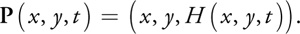
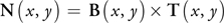
Because we have an explicit function for our surface, we can calculate the surface orientation at any given point directly, rather than depend on finite-differencing techniques. Our binormal B and tangent T vectors are the partial derivatives in the x and y directions, respectively. For any (x, y) in the 2D horizontal plane, the 3D position P on the surface is:
The partial derivative in the x direction is then:
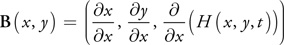
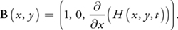
Similarly, the tangent vector is:
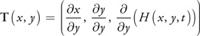
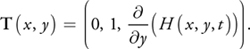
The normal is given by the cross product of the binormal and tangent, as:
Before putting in the partials of our function H, note how convenient the formulas in Equations 3–6 happen to be. The evaluation of two partial derivatives has given us the nine components of the tangent-space basis. This is a direct consequence of our using a height field to approximate our surface. That is, P(x, y).x = x and P(x, y).y = y, which become the zeros and ones in the partial derivatives. It is only valid for such a height field, but is general for any function H(x, y, t) we choose.
For the height function described in Section 1.2.1, the partial derivatives are particularly convenient to compute. Because the derivative of a sum is the sum of the derivatives:
over all waves i.
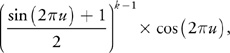
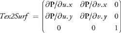
A common complaint about waves generated by summing sine waves directly is that they have too much "roll," that real waves have sharper peaks and wider troughs. As it turns out, there is a simple variant of the sine function that quite controllably gives this effect. We offset our sine function to be nonnegative and raise it to an exponent k. The function and its partial derivative with respect to x are:
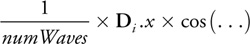
Figure 1-3 shows the wave shapes generated as a function of the power constant k. This is the function we actually use for our texture waves, but for simplicity, we continue to express the waves in terms of our simple sum of sines, and we note where we must account for our change in underlying wave shape.
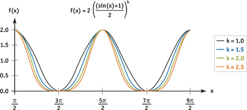
Figure 1-3 Various Wave Shapes
1.2.3 Geometric Waves
We limit ourselves to four geometric waves. Adding more involves no new concepts, just more of the same vertex shader instructions and constants.
Directional or Circular
We have a choice of circular or directional waves, as shown in Figure 1-4. Directional waves require slightly fewer vertex shader instructions, but otherwise the choice depends on the scene being simulated.
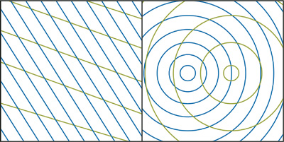
Figure 1-4 Directional and Circular Waves
For directional waves, each of the D i in Equation 1 is constant for the life of the wave. For circular waves, the direction must be calculated at each vertex and is simply the normalized vector from the center C i of the wave to the vertex:
For large bodies of water, directional waves are often preferable, because they are better models of wind-driven waves. For smaller pools of water whose source of waves is not the wind (such as the base of a waterfall), circular waves are preferable. Circular waves also have the nice property that their interference patterns never repeat. The implementations of both types of waves are quite similar. For directional waves, wave directions are drawn randomly from some range of directions about the wind direction. For circular waves, the wave centers are drawn randomly from some finite range (such as the line along which the waterfall hits the water surface). The rest of this discussion focuses on directional waves.
Gerstner Waves
For effective simulations, we need to control the steepness of our waves. As previously discussed, sine waves have a rounded look to them—which may be exactly what we want for a calm, pastoral pond. But for rough seas, we need to form sharper peaks and broader troughs. We could use Equations 8a and 8b, because they produce the desired shape, but instead we choose the related Gerstner waves. The Gerstner wave function was originally developed long before computer graphics to model ocean water on a physical basis. As such, Gerstner waves contribute some subtleties of surface motion that are quite convincing without being overt. (See Tessendorf 2001 for a detailed description.) We choose Gerstner waves here because they have an often-overlooked property: they form sharper crests by moving vertices toward each crest. Because the wave crests are the sharpest (that is, the highest-frequency) features on our surface, that is exactly where we would like our vertices to be concentrated, as shown in Figure 1-5.
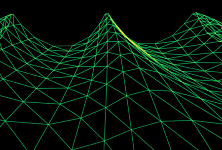
Figure 1-5 Gerstner Waves
The Gerstner wave function is:

Here Qi is a parameter that controls the steepness of the waves. For a single wave i, Qi of 0 gives the usual rolling sine wave, and Qi = 1/(wi Ai ) gives a sharp crest. Larger values of Qi should be avoided, because they will cause loops to form above the wave crests. In fact, we can leave the specification of Q as a "steepness" parameter for the production artist, allowing a range of 0 to 1, and using Qi = Q/(wi Ai x numWaves) to vary from totally smooth waves to the sharpest waves we can produce.
Note that the only difference between Equations 3 and 9 is the lateral movement of the vertices. The height is the same. This means that we no longer have a strict height function. That is, 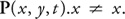 However, the function is still easily differentiable and has some convenient cancellation of terms. Mercifully saving the derivation as an exercise for the reader, we see that the tangent-space basis vectors are:
where:
These equations aren't as clean as Equations 4b, 5b, and 6b, but they turn out to be quite efficient to compute.
A closer look at the z component of the normal proves interesting in the context of forming loops at wave crests. While Tessendorf (2001) derives his "choppiness" effect from the Navier-Stokes description of fluid dynamics and the "Lie Transform Technique," the end result is a variant of Gerstner waves expressed in the frequency domain. In the frequency domain, looping at wave tops can be avoided and detected, but in the spatial domain, we can see clearly what is going on. When the sum Qi x wi x Ai is greater than 1, the z component of our normal can go negative at the peaks, as our wave loops over itself. As long as we select our Qi such that this sum is always less than or equal to 1, we will form sharp peaks but never loops.
Wavelength and Speed
We begin by selecting appropriate wavelengths. Rather than pursue real-world distributions, we would like to maximize the effect of the few waves we can afford. The super-positioning of waves of similar lengths highlights the dynamism of the water surface. So we select a median wavelength and generate random wavelengths between half and double that length. The median wavelength is scripted in the authoring process, and it can vary over time. For example, the waves may be significantly larger during a storm than while the scene is sunny and calm. Note that we cannot change the wavelength of an active wave. Even if it were changed gradually, the crests of the wave would expand away from or contract toward the origin, a very unnatural look. Therefore, we change the current average wavelength, and as waves die out over time, they will be reborn based on the new length. The same is true for direction.
Given a wavelength, we can easily calculate the speed at which it progresses across the surface. The dispersion relation for water (Tessendorf 2001), ignoring higher-order terms, gives:
where w is the frequency and g is the gravitational constant consistent with whatever units we are using (such as 9.8 m/s2), and L is the crest-to-crest length of the wave.
Amplitude
How to handle the amplitude is a matter of opinion. Although derivations of wave amplitude as a function of wavelength and current weather conditions probably exist, we use a constant (or scripted) ratio, specified at authoring time. More exactly, along with a median wavelength, the artist specifies a median amplitude. For a wave of any size, the ratio of its amplitude to its wavelength will match the ratio of the median amplitude to the median wavelength.
Direction
The direction along which a wave travels is completely independent of the other parameters, so we are free to select a direction for each wave based on any criteria we choose. As mentioned previously, we begin with a constant vector that is roughly the wind direction. We then choose randomly from directions within a constant angle of the wind direction. That constant angle is specified at content-creation time, or it may be scripted.
1.2.4 Texture Waves
The waves we sum into our texture have the same parameterization as their vertex cousins, but with different constraints. First, in the texture it is much more important to capture a broad spectrum of frequencies. Second, patterns are more prone to form in the texture, breaking the natural look of the ripples. Third, only certain wave directions for a given wavelength will preserve tiling of the overall texture. Also, note that all quantities here are in units of texels, rather than world-space distance.
We currently use about 15 waves of varying frequency and orientation, taking from two to four passes. Four passes may sound excessive, but they are into a 256x256 render-target texture, rather than over the main frame buffer. In practice, the hit from the fill rate of generating the normal map is negligible.
Wavelength and Speed
Again, we start by selecting wavelengths. We are limited in the range of wavelengths the texture will hold. Obviously, the sine wave must repeat at least once if the texture is to tile. That sets the maximum wavelength at TEXSIZE, where TEXSIZE is the dimension of the target texture. The waves will degrade into sawtooth patterns as the wavelength approaches 4 texels, so we limit the minimum wavelength to 4 texels. Also, longer wavelengths are already approximated by the geometric undulation, so we favor shorter wavelengths in our selection. We typically select wavelengths between about 4 and 32 texels. With the bump map tiling every 50 feet, a wavelength of 32 texels corresponds to about 6 feet. This leaves geometric wavelengths ranging upward from about 4 feet, and texture wavelengths ranging downward from about 6 feet, with just a little overlap.
The wave speed calculation is identical to the geometric form. The exponent in Equations 8a and 8b controls the sharpness of the wave crests.
Amplitude and Precision
We determine the amplitude of each wave as we did with geometric waves, keeping amplitude over wavelength a constant ratio, kAmpOverLen. This leads to an interesting optimization.
Remember that we are not concerned with the height function here; we are only building a normal map. Our lookup texture contains cos(2 u), where u is the texture coordinate ranging from 0 to 1. We store the raw cosine values in our lookup texture rather than in the normals because it is actually easier to convert the cosine into a rotated normal than to store normals and try to rotate them with the texture.
We evaluate the normal of our sum of sines by rendering our lookup texture into a render target. Expressing Equation 7 in terms of u-v space, we have:
where u and v vary from 0 to 1 over the render target. We calculate the inner term,  in the vertex shader, passing the result as the u coordinate for the texture lookup in the pixel shader. The outer terms,
 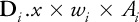 and
and 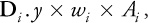 , are passed in as constants. The resulting pixel shader is then a constant times a texture lookup per wave. We note that to use the sharper-crested wave function in Equation 8a, we simply fill in our lookup table with:
instead of cos(2 u), and pass in 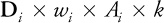 as the outer term.
Using a lookup table here currently provides both speed and flexibility. But just as the relative rates of increase in processor speed versus memory access time have pushed lookup tables on the CPU side out of favor, we can expect the same evolution on the GPU. Looking forward, we expect to be much more discriminating about when we choose a lookup texture over direct arithmetic calculation. In particular, by using a lookup table here, we must regenerate the lookup table to change the sharpness of the waves.
Unlike our approach to the composition of geometric normals in the vertex shader, in creating texture waves we are very concerned with precision. Each component of the output normal must be represented as a biased, signed, fixed-point value with 8 bits of precision. If the surface gets very steep, the x or y component will be larger than the z component and will saturate at 1. If the surface is always shallow, the x and y components will always be close to 0 and suffer quantization errors. In this work, we expect the latter case. If we can establish tight bounds on values for the x and y components, we can scale the normals in the texture to maximize the available precision, and then "un-scale" them when we use them.
Examining the x component of the generated normal, we first see that both the cosine function and the x component of the direction vector range over the interval [–1..1]. The product of the frequency and the amplitude is problematic, because the frequency and amplitude are different for each wave.
Expressing Equation 7 with the frequency in terms of wavelength, we have:
Whereas the height is dominated by waves of greater amplitude, the surface orientation is dominated by waves with greater ratios of amplitude to wavelength.
We first use this result to justify having a constant ratio of amplitude to wavelength across all our waves, reasoning that because we have a very limited number of waves, we choose to omit those of smaller ratios. Second, because of that constant ratio, we know that the x and y components of our waves are limited to having absolute values less than kAmpOverLen x 2, and the total is limited to numWaves x kAmpOverLen x 2. So to preserve resolution during summation, we accumulate:
and scale by numWaves x 2 x kAmpOverLen when we use them.
Direction and Tiling
If the render target has enough resolution to be used without tiling, we can accumulate arbitrary sine functions into it. In fact, we can accumulate arbitrary normal maps into it. For example, we might overlay a turbulent distortion following the movements of a character within the scene. Alternately, we might begin with a more complex function than a single sine wave, getting more wave complexity with the accumulation of fewer "wave" functions. Keep in mind that the power of this technique is in the relative motion of the waves. A complex wave pattern moving as a unit has less realism and impact than simpler waves moving independently.
These additions are relatively straightforward. Getting the render target to tile, however, imposes some constraints on the wave functions we accumulate. In particular, note that a major appeal of circular waves is that they form no repeating patterns. If we want our texture to tile, we need our waves to form repeating patterns, so we limit ourselves to directional waves.
Obviously, a tiling of a texture will tile itself only if the texture is repeated an integer number of times. Also, for a sine wave of given wavelength that tiles, only certain rotations of the texture will still tile. Less obvious, but equally true, is that if each of the rotated sine functions we add in will tile, then the sum of those sine functions also tiles.
Because we rotate and scale the sine functions through the texture transform, we can ensure that both conditions for tiling are met by making certain that the scaled rotation elements of the texture transform are integers. We then translate the wave by adding a phase component into the transform's translation. Note that because the texture is really 1D, we need concern ourselves only with the transformed u coordinate.
1.3 Authoring
We briefly discuss in this section how the water system is placed and modeled offline. Through the modeling of the water mesh, the content author controls the simulation down to the level of the vertex. See Figure 1-6.
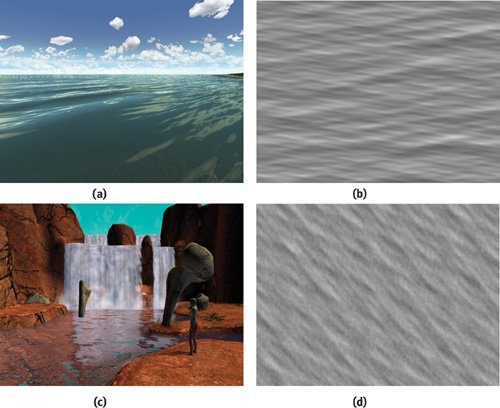
Figure 1-6 Ocean and Pond Water
In our implementation, the mesh data is limited to the tessellation of the mesh, the horizontal positions of each vertex in the mesh, the vertical position of the bottom of the body of water below the vertex, and an RGBA color. Texture coordinates may be explicitly specified or generated on the fly. See Figure 1-7.
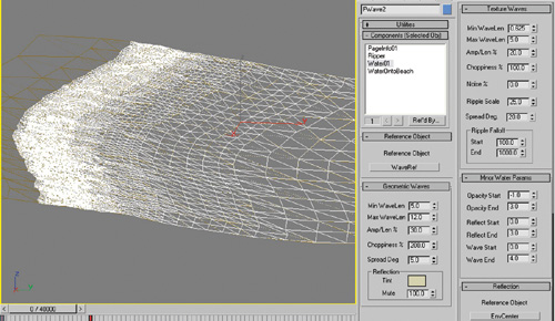
Figure 1-7 The User Interface of the 3ds max Authoring Tool
First, we discuss using the depth of the water at a vertex as an input parameter, from which the shader can automatically modify its behavior in the delicate areas where water meets shore. We also cover some vertex-level system overrides that have proven particularly useful. To prevent aliasing artifacts, we automatically filter out waves for which the sampling frequency of the mesh is insufficient. Finally, we comment on the additional input data necessary when the texture mapping is explicitly specified at content-creation time, rather than implicitly based on a planar mapping over position.
1.3.1 Using Depth
Because the height of the water will be computed, the z component of the vertex position might go unused. We could take advantage of this to compress our vertices, but we choose rather to encode the water depth in the z component instead. More precisely, we put the height of the bottom of the water body in the vertex z component, pass in the height of the water table as a constant, and have the depth of the water available with a subtraction. Again, this assumes a constant-height water table. To model something like a river flowing downhill, we need an explicit 3D position as well as a depth for each vertex. In such a case, the depth may be calculated offline using a simple ray cast from water surface to riverbed, or it can be explicitly authored as a vertex color, but in any case, the depth must be passed in as an additional part of the vertex data.
We use the water depth to control the opacity of the water, the strength of the reflection, and the amplitude of the geometric waves. For example, one pair of input parameter for the system is a depth at which the water is transparent and a depth at which it is at maximum opacity. This might let the water go from transparent to maximum opacity as the depth goes from 0 at the shore to 3 feet deep. This is a very crude modeling of the fact that shallow water tints the bottom less than deep water does. Having the depth of the water available also allows for more sophisticated modeling of light transmission effects.
Attenuating the amplitude of the geometric waves based on depth is as much a matter of practicality as physical modeling. Attenuating out the waves where the water mesh meets the water plane allows for water vertices to be "fixed" where the mesh meets steep banks. It also gives a gradual die-off of waves coming onto a shallow shore. Because we constrain our vertices never to go below their input height, attenuating the waves to zero slightly above the water plane allows waves to lap up onto the shore, while enabling us to control how far up the shore they can go.
1.3.2 Overrides
For the most part, the system "just works," processing all vertices identically. But there are valid occasions for the content author to override the system behavior on a per-vertex basis. We encode these overrides as the RGB vertex color. Left at their defaults of white, these overrides pass all control to the simulation. Bringing down a channel to zero modulates an effect.
The red component governs the overall transparency, making the water surface completely transparent when red goes to zero. Green modulates the strength of the reflection on the surface, making the water surface matte when green is zero. Blue limits the opacity attenuation based on viewing angle, which affects the Fresnel term. An alternate use of one of these colors would be to scale the horizontal components of the calculated per-pixel normal. This would allow some areas of the water to be rougher than others, an effect often seen in bays.
1.3.3 Edge-Length Filtering
If you are already familiar with signal-processing theory, then you readily appreciate that the shortest wavelength we can use to undulate our mesh depends on how finely tessellated the mesh is. From the Nyquist theorem, we need our vertices to be separated by at most half the shortest wavelength we are using. If that doesn't seem obvious, refer to Figure 1-8, which gives an intuitive, if nonrigorous, explanation of the concept. As long as the edges of the triangles in the mesh are short compared to the wavelengths in our height function, the surface will look good. When the edge lengths get as long as, or longer than, half the shortest wavelengths in our function, we see objectionable artifacts.
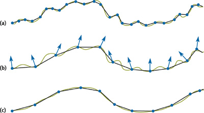
Figure 1-8 Matching Wave Frequencies to Tessellation
One reasonable and common approach is to decide in advance what the shortest wavelength in our height function will be and then tessellate the mesh so that all edges are somewhat shorter than that wavelength. In this work we take another approach: We look at the edge lengths in the neighborhood of a vertex and then filter out waves that are "too short" to be represented well in that neighborhood.
This technique has two immediate benefits. First, any wavelengths can be fed into the vertex processing unit without undesirable artifacts, regardless of the tessellation of the mesh. This allows the simulation to generate wavelengths solely based on the current weather conditions. Any wavelengths too small to undulate the mesh are filtered out with an attenuation value that goes from 1 when the wavelength is 4 times the edge length, to 0 when the wavelength is twice the edge length. Second, the mesh need not be uniformly tessellated. More triangles may be devoted to areas of interest. Those areas of less importance, with fewer triangles and longer edges, will be flatter, but they will have no objectionable artifacts. An example would be modeling a cove heavily tessellated near the shore, using larger and larger triangles as the water extends out to the horizon.
1.3.4 Texture Coordinates
Usually, texture coordinates need not be specified. They are easily derived from the vertex position, based on a scale value that specifies the world-space distance that a single tile of the normal map covers.
In some cases, however, explicit texture coordinates can be useful. One example is having the water flow along a winding river. In this case, the explicit texture coordinates must be augmented with tangent-space vectors, to transform the bump-map normals from the space of the texture as it twists through bends into world space. These values are automatically calculated offline from the partial derivatives of the position with respect to texture coordinate, as is standard with bump maps. The section "Per-Pixel Lighting" in Engel 2002 gives a practical description of generating tangent-space basis vectors using DirectX.
1.4 Runtime Processing
Let's consider the processing in the vertex and pixel shaders here at a high level. Refer to the accompanying source code for specifics. With the explanations from the previous sections behind us, the processing is fairly straightforward. Only one subtle issue remains unexplored.
Having a dynamic, undulating geometric surface, and a complex normal map of interacting waves, we need only to generate appropriate bump-environment mapping parameters to tie the two together. Those parameters are the transform to take our normals from texture space to world space, and an eye vector to reflect off our surface into our cubic environment map. We derive those first and then walk through the vertex and pixel processing.
1.4.1 Bump-Environment Mapping Parameters
Tangent-Space Basis Vectors
We can compute space basis vectors from the partial derivatives of our water surface function. Equations 10, 11, and 12 give us the binormal B, the tangent T, and the normal N.
We stack those values into three vectors (that is, output texture coordinates) to be used as a row-major matrix, so our matrix will be:
Except for where we got the basis vectors, this is the usual transform for bump mapping. It accounts for our surface being wavy, not flat, transforming from the undulating surface space into world space. If the texture coordinates for our normal map are implicit—that is, derived from the vertex position—then we can assume that there is no rotation between texture space and world space, and we are done. If we have explicit texture coordinates, however, we must take into account the rotations as the texture twists along the river.
Having computed  P/ u and P/ v offline, we use these to form a rotation matrix to transform our texture-space normals into surface-space normals.
This is clearly a rotation in the horizontal plane, which we expect because we collapsed the water mesh to z = 0 before computing the gradients. In the more general case where the base surface is not flat, this would be a full 3x3 matrix. In either case, order is important, so our concatenated matrix is Surf2World x Tex2Surf.
If we want to rescale the x and y components of our normals, we must take one final step. We might want to rescale the components because we had scaled them to maximize precision when we wrote them to the normal map. Or we might want to rescale them based on their distance from the camera, to counter aliasing. In either case, we want the scale to be applied to the x and y components of the raw normal values, before either of the preceding transforms. Then, assuming a uniform scale factor s, our scale matrix and final transform are:
Eye Vector
We typically use the eye-space position of the vertex as the eye vector on which we base our lookup into the environment map. This effectively treats the scene in the environment map as infinitely far away.
If all that is reflected in the water is more or less infinitely far away—for example, a sky dome—then this approximation is perfect. For smaller bodies of water, however, where the reflections show the objects on the opposite shore, we would like something better.
Rather than at an infinite distance, we would like to assume the reflected features are at a uniform distance from the center of our pool. That is, we will project the environment map onto a sphere of the same radius as our pool, centered about our pool. Brennan 2002 describes a very clever and efficient approximation for this. We offer an alternate approach.
Figure 1-9 gives an intuitive feel for the problem as well as the solution. Given an environment map generated from point C, the camera is now at point E looking at a vertex at point P. We would like our eye vector to pass from E through P and see the object at A in the environment map. But the eye vector is actually relative to the point from which the environment map was generated, so we would sample the environment map at point B.
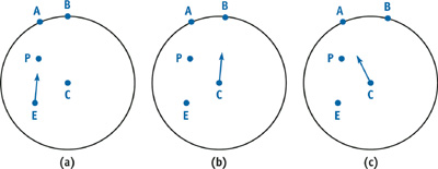
Figure 1-9 Correction of the Eye Vector
We would like to calculate an eye vector that will take us from C to A. We can find A as the point where our original eye vector intersects the sphere, and then our corrected eye vector is A - C. Because A is on the sphere of radius r, and A = E + (P - E)t, we have:
This expands out to:
0 = (P - E)2 · t 2 - 2(P - E)(E - C) · t + (E - C)2 - r 2.
We solve for t using the quadratic equation, giving:
Here we make some substitutions:
Substituting in and discarding the lesser root gives us:
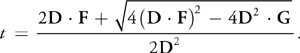
Canceling our 2s and recognizing that D 2 = 1 (it's normalized), gives us:
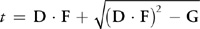
and
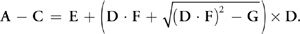
We already have D, the normalized eye vector, because we use it for attenuating the water opacity based on viewing angle. F and G are constants. So calculating t and our corrected eye vector, although it started out ugly, requires only five arithmetic operations. This underlines a powerful point made in Fernando and Kilgard 2003, namely, that collapsing values that are constant over a mesh into shader constants can bring about dramatic and surprising optimizations within the shader code.
Because we have essentially intersected a ray with a sphere, this method will obviously fail if that ray does not intersect the sphere. This possibility doesn't especially concern us, however. There will always be a real root if either the eye position or the vertex position lies within the sphere, and since the sphere encompasses the scenery around the body of water, it is safe to constrain the water vertices to lie within the sphere.
Note that where the surroundings reflected off a body of water are not well approximated by a mapping onto a sphere, or where the surroundings are too dynamic to be captured by a static environment map, a projective method such as the one described in Vlachos et al. 2002 might be preferable.
1.4.2 Vertex and Pixel Processing
We begin by evaluating the sine and cosine functions for each of our four geometric waves.
Before summing them, we subtract our input vertex Z from our water-table height constant to get the depth of the water at this vertex. That depth forms our first wave-height attenuation factor by some form of interpolation between input constant depths.
Because we have stored the minimum edge length in the neighborhood of this vertex, we now use that to attenuate the heights of the waves independently, based on wavelength. That attenuation will filter out waves as the edge length gets as long as a fraction of the wavelength.
Explicit texture coordinates are passed through as is. Implicit coordinates are simply a scaling of the x and y positions of the vertex. The transformation from texture space to world space is calculated as described in Section 1.4.1. The scale value used is the input constant numWaves x 2 x kAmpOverLen, as described in the "Amplitude and Precision" subsection of Section 1.2.4. The scale value is modulated by another scale factor that goes to zero with increasing distance from the vertex to the eye. This causes the normal to collapse to the geometric surface normal in the distance, where the normal map texels are much smaller than pixels. The eye vector is computed as the final piece needed for bump environment mapping.
We emit two colors per vertex. The first is the color of the water proper. The second will tint the reflections off the water. The opacity of the water proper is modulated first as a function of depth, generally getting more transparent in shallows. Then it is modulated based on the viewing angle, so that the water is more transparent when viewed straight on than when viewed at a glancing angle. A per-pixel Fresnel term, as well as other more sophisticated effects, could be calculated by passing the view vector into the pixel shader, rather than computing the attenuation at the vertex level. The reflection color is also modulated based on depth and viewing angle, but independently to provide separate controls for when and how transparent the reflection gets.
In the pixel processing stage, there is little left to do. A simple bump lookup into an environment map gives the reflection color. We currently look up into a cubic environment map, but the projected planar environment maps described in Vlachos et al. 2002 would be preferable in many situations. The reflected color is modulated and added to the color of the water proper. The pixel is emitted and alpha-blended to the frame buffer.
1.5 Conclusion
Water simulation makes an interesting topic in the context of vertex and pixel shaders, partly because it leverages such distinct techniques into a cohesive system. The work described here combines enhanced bump environment mapping with the evaluation of complex functions in both vertex and pixel shaders. We hope this chapter will prove useful in two ways: First, by detailing the physics and math behind what is frequently thought of as an ad hoc system, we hope we have shown how the system itself becomes more extensible. More and better wave functions on the geometric as well as the texture side could considerably improve the system, but only with an understanding of how the original waves were used. Second, the system as described generates a robust, dynamic, controllable, and realistic water surface with minimal resources. The system requires only vs.1.0 and ps.1.0 support. On current and future hardware, that leaves a lot of resources to carry forward with more sophisticated effects in areas such as light transport and reaction to other objects.
1.6 References
Jeff Landers has a good bibliography of water techniques on the Darwin 3D Web site: http://www.darwin3d.com/vsearch/FluidSim.txt
And another good one, on the Virtual Terrain Project Web site: http://www.vterrain.org/Water/index.html
Brennan, Chris. 2002. "Accurate Reflections and Refractions by Adjusting for Object Distance." In ShaderX, edited by Wolfgang Engel. Wordware. http://www.shaderx.com
Engel, Wolfgang. 2002. "Programming Pixel Shaders." In ShaderX, edited by Wolfgang Engel. Wordware. http://www.shaderx.com
Enright, Douglas, Stephen Marschner, and Ronald Fedkiw. 2002. "Animation and Rendering of Complex Water Surfaces." In Proceedings of SIGGRAPH 2002. Available online at http://graphics.stanford.edu/papers/water-sg02/water.pdf
Fernando, Randima, and Mark J. Kilgard. 2003. The Cg Tutorial. Addison-Wesley.
Isidoro, John, Alex Vlachos, and Chris Brennan 2002. "Rendering Ocean Water." In ShaderX, edited by Wolfgang Engel. Wordware. http://www.shaderx.com
Laeuchli, Jesse. 2002. "Simple Gerstner Wave Cg Shader." Online article. Available online at http://www.cgshaders.org/shaders/show.php?id=46
Tessendorf, Jerry. 2001. "Simulating Ocean Water." In Proceedings of SIGGRAPH 2001. Course slides available online here at online.cs.nps.navy.mil
Vlachos, Alex, John Isidoro, and Chris Oat. 2002. "Rippling Reflective and Refractive Water." In ShaderX, edited by Wolfgang Engel. Wordware. http://www.shaderx.com
Yann, L. 2003. "Realistic Water Rendering." E-lecture. Available online at http://www.andyc.org/lecture/viewlog.php?log=Realistic%20Water%20Rendering,%20by%20Yann%20L
Copyright
Many of the designations used by manufacturers and sellers to distinguish their products are claimed as trademarks. Where those designations appear in this book, and Addison-Wesley was aware of a trademark claim, the designations have been printed with initial capital letters or in all capitals.
The authors and publisher have taken care in the preparation of this book, but make no expressed or implied warranty of any kind and assume no responsibility for errors or omissions. No liability is assumed for incidental or consequential damages in connection with or arising out of the use of the information or programs contained herein.
The publisher offers discounts on this book when ordered in quantity for bulk purchases and special sales. For more information, please contact:
U.S. Corporate and Government Sales
(800) 382-3419
corpsales@pearsontechgroup.com
For sales outside of the U.S., please contact:
International Sales
international@pearsoned.com
Visit Addison-Wesley on the Web: www.awprofessional.com
Library of Congress Control Number: 2004100582
GeForce™ and NVIDIA Quadro® are trademarks or registered trademarks of NVIDIA Corporation.
RenderMan® is a registered trademark of Pixar Animation Studios.
"Shadow Map Antialiasing" © 2003 NVIDIA Corporation and Pixar Animation Studios.
"Cinematic Lighting" © 2003 Pixar Animation Studios.
Dawn images © 2002 NVIDIA Corporation. Vulcan images © 2003 NVIDIA Corporation.
Copyright © 2004 by NVIDIA Corporation.
All rights reserved. No part of this publication may be reproduced, stored in a retrieval system, or transmitted, in any form, or by any means, electronic, mechanical, photocopying, recording, or otherwise, without the prior consent of the publisher. Printed in the United States of America. Published simultaneously in Canada.
For information on obtaining permission for use of material from this work, please submit a written request to:
Pearson Education, Inc.
Rights and Contracts Department
One Lake Street
Upper Saddle River, NJ 07458
Text printed on recycled and acid-free paper.
5 6 7 8 9 10 QWT 09 08 07
5th Printing September 2007
- Contributors
- Copyright
- Foreword
- Part I: Natural Effects
-
- Chapter 1. Effective Water Simulation from Physical Models
- Chapter 2. Rendering Water Caustics
- Chapter 3. Skin in the "Dawn" Demo
- Chapter 4. Animation in the "Dawn" Demo
- Chapter 5. Implementing Improved Perlin Noise
- Chapter 6. Fire in the "Vulcan" Demo
- Chapter 7. Rendering Countless Blades of Waving Grass
- Chapter 8. Simulating Diffraction
- Part II: Lighting and Shadows
-
- Chapter 9. Efficient Shadow Volume Rendering
- Chapter 10. Cinematic Lighting
- Chapter 11. Shadow Map Antialiasing
- Chapter 12. Omnidirectional Shadow Mapping
- Chapter 13. Generating Soft Shadows Using Occlusion Interval Maps
- Chapter 14. Perspective Shadow Maps: Care and Feeding
- Chapter 15. Managing Visibility for Per-Pixel Lighting
- Part III: Materials
- Part IV: Image Processing
- Part V: Performance and Practicalities
-
- Chapter 28. Graphics Pipeline Performance
- Chapter 29. Efficient Occlusion Culling
- Chapter 30. The Design of FX Composer
- Chapter 31. Using FX Composer
- Chapter 32. An Introduction to Shader Interfaces
- Chapter 33. Converting Production RenderMan Shaders to Real-Time
- Chapter 34. Integrating Hardware Shading into Cinema 4D
- Chapter 35. Leveraging High-Quality Software Rendering Effects in Real-Time Applications
- Chapter 36. Integrating Shaders into Applications
- Part VI: Beyond Triangles
- Preface