
Single-cell sequencing has become one of the most prominent technologies used in biomedical research. Its ability to decipher changes in the transcriptome and epigenome on a cell level has enabled researchers to gain valuable new insights. As a result, single-cell experiments have grown in size and complexity by a factor of over 100, with experiments involving more than 1 million cells becoming increasingly common.
However, the resulting data must be analyzed in a highly iterative process. It is crucial that fast algorithms are used for these iterative steps to enable quick turnaround times.
For more consistent single-cell analysis using Python, developers at scverse have worked toward building an entire ecosystem to help researchers perform analyses. At the core of this ecosystem lies a data structure that maintains annotations of various transformations throughout the data processing pipeline during single-cell analysis.
AnnData, a Python package for handling annotated data matrices in memory and on disk, is the core structure used in the Scanpy library, which is the main single-cell analysis suite within the scverse ecosystem. Scanpy builds on top of other libraries common to the PyData ecosystem—such as NumPy, SciPy, Numba, and Scikit-learn—for just about all of the typical analysis steps.
However, Scanpy algorithms are mostly CPU-based and slow down significantly with larger experiments. The highly iterative nature of the single-cell analysis process only compounds this problem.
GPUs for single-cell analysis
General feasibility of running downstream single-cell RNA sequencing (scRNA-seq) analysis on the GPU with RAPIDS and Scanpy has been shown in Accelerating Single-Cell Genomic Analysis with GPUs. This work resulted in the rapids-single-cell-examples GitHub repo, which contains a series of example notebooks written by the RAPIDS and NVIDIA Parabricks teams. RAPIDS is an open-source suite of libraries for GPU-accelerated data science with Python. Parabricks is a free suite of GPU-accelerated, industry-standard genomic analysis tools based on deep learning.
While these example notebooks demonstrate a few typical single-cell RNA workflows on the GPU, they were never intended for daily use nor as a GPU-accelerated replacement for libraries like Scanpy.
Drawing inspiration from prior work on rapids-single-cell-examples is an emerging library called rapids-singlecell, a GPU-accelerated tool for scRNA analysis. This tool aims to be a daily drivable single-cell analysis suite that is compatible with the scverse ecosystem. It uses RAPIDS and CuPy to provide GPU-accelerated functions that are near-drop-in replacements for the corresponding functions in Scanpy.
On average, users can expect performance to increase between 10x and 20x by using rapids-singlecell. For more details, see Accelerating Single Cell Genomic Analysis Using RAPIDS.
Faster single-cell analysis using RAPIDS
rapids-singlecell follows a similar usability model as the scverse Python libraries. It is also written in Python but puts many of the performance-critical pieces on the GPU, hiding all of the complexities that are normally associated with writing CUDA applications (the language typically used to write accelerated algorithms for NVIDIA GPUs).
rapids-singlecell consists of five categories, which are described in the sections that follow. Each category accelerates a different piece of the typical single cell analysis workflow.
For more information, including the various APIs offered by rapids-singlecell, see the rapids-singlecell documentation.
cunnData
The AnnData, or annotated data object, is a widely used data structure for handling single-cell RNA sequencing data. In contrast, cunnData is a minimized and lightweight version of the AnnData object for the GPU that replaces the scverse standard for preprocessing (Figure 1). Instead of storing the count matrix .X on the CPU, cunnData stores it on the GPU as CuPy sparse matrices. This makes it faster and more efficient to perform computations on the count matrix. It also contains annotation dataframes for cells (.obs attribute) and genes (.var attribute), which store additional information such as cell type and gene names.
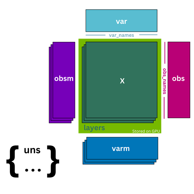
cunnData also includes additional features, such as the ability to store different versions of the count matrix, such as raw integer counts, in .Layers. Unlike AnnData, which stores .Layers in Host (CPU) memory, cunnData also stores .Layers on the GPU, reducing the need to copy data from the host to GPU memory and enabling accelerated computations.
cunnData supports unstructured annotations in the .uns attribute, as well as multidimensional annotations of cells and genes in the .obsm and .varm attributes, which are stored in the host memory. These annotations enable users to include additional information about their data, such as spatial coordinates or principal component analysis (PCA) embeddings.
Similarly, cunnData supports slicing like AnnData. These slices, however, are always full copies of the original data, as opposed to views. Overall, cunnData enables a faster approach to preprocessing scRNA-seq data compared to the more feature-rich CPU-bound AnnData object.
The Python snippet below demonstrates the conversion of an AnnData object (a standard data structure for handling single-cell RNA sequencing data) into a cunnData object.
import scanpy as sc
import rapids_singlecell as rsc
adata = sc.read("PATH TO DATASET")
cudata = rsc.cunnData.cunnData(adata=adata)
Preprocessing
The preprocessing functions are stored in cunnData_funcs, which provides accelerated alternatives to the Scanpy preprocessing functions. These functions work on the cunnData object and use RAPIDS cuML and CuPy to dramatically accelerate Scanpy functions based on Scikit-learn, Numpy and SciPy.
Filtering cells and genes can be accomplished with filter_cells and filter_genes functions, respectively. Quality control is handled with the calculate_qc_metrics function.
# Basic QC rapids-singlecell
rsc.pp.flag_gene_family(cudata,gene_family_name="MT", gene_family_prefix="mt-")
rsc.pp.calculate_qc_metrics(cudata,qc_vars=["MT"])
cudata = cudata[cudata.obs["n_genes_by_counts"] > 500]
cudata = cudata[cudata.obs["pct_counts_MT"] < 20]
rsc.pp.filter_genes(cudata,min_count=3)
To normalize your data, cunnData_funcs provides GPU alternatives to the normalize_total, log1p, and the recently introduced normalize_pearson_residuals functions from Scanpy. Annotating highly variable genes is accelerated for all flavors supported in Scanpy (including seurat, cellranger, seurat_v3, pearson_residuals), as well as poisson_gene_selection, which is adapted from scvi-tools.
# log normalization and highly variable gene selection
cudata.layers["counts"] = cudata.X.copy()
rsc.pp.normalize_total(cudata,target_sum=1e4)
rsc.pp.log1p(cudata)
rsc.pp.highly_variable_genes(cudata,n_top_genes=5000,flavor="seurat_v3",layer = "counts")
cudata = cudata[:,cudata.var["highly_variable"]==True]
The regress_out function, used to remove unwanted sources of variation, is accelerated with the cuML linear regression estimator. It also supports multitarget regression, which was introduced in cuML in version 22.12, while staying backwards compatible with prior versions.
Principal component analysis wraps cuML PCA, Truncated SVD, and Incremental PCA to give you the same options offered by Scanpy. With the PCA version in cunnData_funcs, you can choose which layer you want to use for the analysis, an additional feature not currently supported by the scanpy PCA function.
# Regression, scaling and PCA
rsc.pp.regress_out(cudata,keys=["total_counts", "pct_counts_MT"])
rsc.pp.scale(cudata,max_value=10)
rsc.pp.pca(cudata, n_comps = 100)

sc.pl.pca_variance_ratio(cudata, log=True,n_pcs=100)
cunndata_funcs can accelerate preprocessing by a factor of 10 to 20x (Tables 1-3). After preprocessing, the cunnData object is transformed into an AnnData object.
adata_preprocessed = cudata.to_AnnData()
Tools
scanpy_gpu provides functions that work on the AnnData object, with the goal of providing accelerated functions. To keep the syntax as close as possible between Scanpy and rapids-singlecell, metadata is also written to the .uns attribute. This attribute is useful for storing trained parameters such as the variance ratio, which is computed during the PCA computation. scanpy_gpu provides a PCA function for the AnnData object equivalent to cunnData_funcs.
Scanpy already includes support for computing UMAP and nearest neighbors on the GPU using cuML. scanpy_gpu extends Scanpy GPU support by adding more algorithms, such as accelerated graph-based clustering using Leiden and Louvain from cuGraph, as well as the Force Atlas 2 algorithm for visually laying out graph data. scanpy_gpu also uses PCA and kernel density estimation (KDE) from cuML and diffusion maps are computed using the CuPy library in a similar manner to how Scanpy uses SciPy and Numpy for scientific computing.
For batch correction, scanpy_gpu provides a GPU port of Harmony Integration, called harmony_gpu. PyMDE (minimum distortion embedding), a function that enables embedding single-cell data while jointly learning the graph and the low-dimensional representation in a probabilistic manner, has also been adapted from scvi-tools.
The near-drop-in replacement nature of rapids-singlecell relies on Scanpy for visualization. It is intuitive to use Scanpy for plotting directly within the scverse framework.
Decoupler
The decoupler tool uses a unified framework to implement several different statistical methods with a focus on biological activity. (Cellular, molecular, and physiological processes in living organisms, for example, gene sets and transcription factors activity.) decoupler_gpu re-implements and accelerates the weighted sum (run_wsum) and multivariate linear model (run_mlm) methods. The GPU port in rapids-singlecell uses the same nets/models as decoupler. Table 1 shows a performance increase of up to 37x for wsum.
Squidpy developments
rapids-singlecell is continually expanding with new accelerated functions for the scverse ecosystem. Comprehensive tests have been added to the library to ensure the correctness and reliability of the code. Squidpy enables detailed analysis and visualization of spatial molecular data. It facilitates understanding of complex cell interactions and spatial patterns, greatly contributing to the expansion of the scverse ecosystem.
Some functions have been accelerated with rapids-singlecell. Spatial auto-correlation with Moran’s I and Geary’s C promises a performance increase of up to 100x. The ligand-receptor (ligrec) interaction analysis in Squidpy has also been optimized and accelerated, resulting in a performance increase of more than 10x.
Benchmarks
Our benchmark results show that using GPU acceleration with the rapids-singlecell package and the decoupler functions can significantly improve the performance of scRNA-seq analysis.
For example, running a sample rapids-singlecell notebook with about 90 K cells end-to-end on a server node with two AMD Epyc Milan 7543, 500 GB memory, and an NVIDIA A100 80 GB GPU was completed in just 51 seconds using the rapids-singlecell package, compared to 1,106 seconds with the traditional scanpy CPU workflow.
Similarly, the decoupler functions also demonstrated significant speed improvements, with the mlm function running in just 12 seconds on the GPU compared to 83 seconds on the CPU, and the wsum method completing in just 26 seconds on the GPU compared to 16 minutes and 10 seconds on the CPU.
Overall, these results demonstrate the potential for GPU acceleration to make scRNA-seq analysis faster and more efficient. These benchmark results are summarized in Table 1.
| Function | CPU | GPU | Speedup |
| Whole notebook(excluding decoupler functions) | 1,106 s (18.5 min) | 51 s | 21x |
| Preprocessing | 74 s | 8 s | 9x |
| Regress out | 27 s | 1.6 s | 16x |
| PCA | 35 s | 0.7 s | 50x |
| HVG (Seurat v3) | 3.2 s | 0.4 s | 8x |
| Harmony | 417 s | 18 s | 23x |
| Neighbors | 22 s | 5.1 s | 4.3x |
| UMAP | 36 s | 0.4 s | 90x |
| TSNE | 133 s | 2.4 s | 55x |
| Louvain | 17 s | 0.6 s | 28x |
| Leiden | 14 s | 0.2 s | 70x |
| Logistic regression | 58 s | 3.7 s | 15x |
| Draw graph (FA2) | 256 s | 0.3 s | 850x |
| run_mlm (DoRothEA) | 83 s | 12 s | 7x |
| Run_wsum (PROGENy) | 970 s (16 min) | 26 s | 37x |
In addition to the previous benchmark results, running a sample rapids-singlecell notebook with 500 K cells on the server node takes about 2 minutes when using rapids-singlecell. The same analysis takes about 41 minutes on the CPU.
Furthermore, using pearson_residuals for highly variable gene selection and normalization can also be accelerated using GPUs, providing additional speed improvements in scRNA-seq analysis. These benchmark results are summarized in Table 2.
rapids-singlecell is not only capable of accelerating single-cell data analysis on high-end server nodes, but also on consumer-grade hardware. Running the same notebook end-to-end with 50,000 cells on a desktop system with an AMD 5950x CPU, 64 GB memory, and an NVIDIA RTX 3090 GPU, takes around 5 minutes using rapids-singlecell. Although the system was using the RAPIDS Memory Manager (RMM) and unified memory to oversubscribe the GPUs memory, it saw a significant speedup compared to the CPU server. These benchmark results are summarized in Table 2.
| Function | CPU | GPU (A100) | GPU (3090) | Speedup |
| Whole notebook(excluding PR functions) | 2,460 s (41 min) | 110 s | 290 s | 22x |
| Preprocessing | 305 s | 28 s | 169 s | 10x |
| HVG (Seurat v3) | 48 s | 1.5 s | 13 s | 32x |
| Regress out | 104 s | 5.1 s | 16 s | 20x |
| scale | 8.4 s | 1.3 s | 5 s | 6.4x |
| PCA | 86 s | 3.7 s | 35 s | 23x |
| Neighbors | 74 s | 17.1 s | 18.3 s | 4.3x |
| UMAP | 281 s (4.6 min) | 6.7 s | 7.6 s | 60x |
| TSNE | 786 s (13 min) | 10 s | 12.9 s | 105x |
| Louvain | 283 s (4.5 min) | 4.5 s | 5.7 s | 62x |
| Leiden | 282 s (4.5 min) | 0.6 s | 0.9 s | 470x |
| Logistic regression | 452 s (7.5 min) | 33 s | 63 s | 13x |
| Diffusion map | 30 s | 0.75 s | 1.3 s | 40x |
| HVG (PR) | 104 s | 2.1 s | 15.6 s | 50x |
| Normalize (PR) | 22 s | 0.3 s | 1 s | 73x |
Running the same sample notebook (Table 1) with about 90 K cells end-to-end on the desktop system takes only 48 seconds when using rapids-singlecell. In comparison, the traditional scanpy CPU workflow takes 774 seconds. The accelerated decoupler functions also demonstrate significant speed improvements on consumer-grade hardware. These benchmark results are summarized in Table 3.
| Function | CPU | GPU | Speedup |
| Whole notebook(excluding decoupler functions) | 774 s (13 min) | 48 s | 16x |
| Preprocessing | 114 s | 6 s | 19x |
| Regress out | 62 s | 1.6 s | 39x |
| PCA | 42 s | 0.7 s | 60x |
| HVG (Seurat v3) | 2.7s | 0.4 s | 6.7x |
| Harmony | 175 s | 21.7 s | 8x |
| Neighbors | 14.9 s | 4.6 s | 3.2x |
| UMAP | 31 s | 0.3 s | 103x |
| TSNE | 95 s | 1.4 s | 68x |
| Louvain | 9.3 s | 0.5 s | 18x |
| Leiden | 13.2 s | 0.1 s | 130x |
| Logistic regression | 76 s | 3.75 s | 20x |
| Draw graph (FA2) | 191 s | 0.23 s | 830x |
| run_mlm (DoRothEA) | 55 s | 12 s | 4.5x |
| Run_wsum (PROGENy) | 690 s (11.5 min) | 28 s | 26x |
Installation
There are multiple methods for installing rapids-singlecell. The easiest method is to use one of the provided yaml files provided within the GitHub repository. These set up the entire environment with everything needed for running the example notebooks.
conda create -f conda/rsc_rapids_23.02.yml
You can also install rapids-singlecell from PyPI into a Conda environment and install RAPIDS from Conda. The default installer does not include RAPIDS or CuPy. Scanpy is also excluded because it is technically not necessary.
pip install rapids-singlecell
Finally, you can install the entire library, including the RAPDIS dependencies, from PyPI using the new experimental PyPI packages from RAPIDS. However, this method of installation requires the user to properly set up CUDA so that it can be found by RAPIDS and CuPy.
To do this, you can use the following command:
pip install 'rapids-singlecell[rapids]’ --extra-index-url=https://pypi.nvidia.com
Conclusion
With the rapids-singlecell library, it is possible to run the complete analysis of 500 K cells in less time than it takes a CPU to compute only its UMAP embedding. Therefore, it enables a much faster iterative process in single-cell data analysis stages.
rapids-singlecell also enables the bioinformatician to analyze the data with a physician or biologist in real time, leading to better collaboration and interpretation of the data. In our experience, it is possible to analyze 200 K cells without any issues, even on a consumer-class 3090 series graphics card. Even better, RMM enables the GPU memory to be oversubscribed and spilled to the main memory, enabling scales well over 500 K cells.
With the datacenter-class NVIDIA A100 80 GB GPU, you can analyze matrices containing as many as 231-1 (approximately 2.15 billion) non-zero counts. (Note that this is the current limit imposed by the CuPy 32-bit integer-based indexing for sparse matrix calculations.) This powerful capability enables users to analyze datasets with over 1 million cells.
The upwards of 20x speedup that rapids-singlecell provides enables researchers to focus more on analyzing and interpreting their single-cell data, rather than waiting for lengthy computational processes. In the true spirit of RAPIDS, this ultimately enhances productivity and fosters new insights into cellular biology that were not possible before.
