Sensor simulation is a critical tool to address the gaps in real-world data for autonomous vehicle (AV) development. However, it is only effective if sensor models accurately reflect the physical world.
Sensors can be either passive, such as cameras—or active, sending out either an electromagnetic wave (lidar, radar) or an acoustic wave (ultrasonic) to generate the sensor output. When modeled in simulation, each modality must be validated against its real-world counterpart.
In previous posts, we detailed the validation process for camera and lidar models in NVIDIA DRIVE Sim. See Validating NVIDIA DRIVE Sim Camera Models and Validating NVIDIA DRIVE Sim Lidar Models. This post will cover radar, an essential sensor for obstacle detection and avoidance.
There are multiple ways to approach radar validation. You can compare how an AV stack trained on real-world data behaves when encountering synthetic radar data, for example. Or, you can compare synthetic radar data to its physical counterpart in real-world experiments.
Validating the model with an AV stack only evaluates its ability to the extent of triggering the AV function, which tests for a lower fidelity ceiling. For this reason, we will focus on the second approach.
Radar sensor pipeline
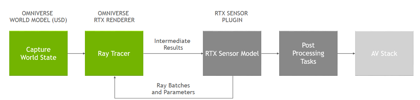
Radar sensors emit radio waves that reflect off objects in the scene and return to the sensor. The received signal then undergoes multiple processing stages that identify the returns from real objects and filter noises. These returns are then presented as a point cloud of the environment.
Such postprocessing methods are typically part of a sensor maker’s intellectual property, and thus NVIDIA DRIVE Sim sensor models aim to approximate them. Sensor suppliers in the DRIVE Sim ecosystem can include the exact implementations of their entire pipelines, including postprocessing.
DRIVE Sim uses ray tracing to model active sensors. Rays that embed the radar radiation pattern are fired into the scene. For each ray that hits an object in the 3D scene, secondary rays are created for reflections and transmissions based on the hit material’s wavelength-dependent properties. The materials in DRIVE Sim use bidirectional scattering distribution functions (BSDF). This enables simulating multipath effects.
DRIVE Sim ray tracing is time-aware. Each ray has its own timestamp and sees a different environment and sensor position to match that time. This enables simulating time-based effects, such as rolling shutter and Doppler.
For radar, after the stopping criteria for ray tracing are met, the sensor model consolidates the returns and processes them. Our radar model accounts for the sensor’s field of view (FOV), antenna directivity, resolutions, ambiguities, and the radar’s sensitivity pattern. A constant false alarm rate (CFAR) algorithm is used to extract valid detections over a simulated noise baseline. The detections are then encoded with the exact communication protocol as the real sensor to serve hardware-in-the-loop use cases.
Radar validation
To validate the DRIVE Sim radar model, we designed three scenarios based on the technical product specification (TPS) of the real radar. The goal was to test various components of the radar sensor’s performance, including its detection capability over its FOV, separation capability, and accuracy in dynamic conditions. Then, we created a digital twin environment in simulation, collecting the equivalent data in DRIVE Sim for detailed analysis.
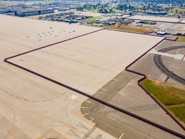
Data collection environment
For the data collection environment, we opted for an open spacious area—the Transportation Research Center in California. In this environment, we could minimize noise and unwanted reflections to simplify digital twin construction in DRIVE Sim.
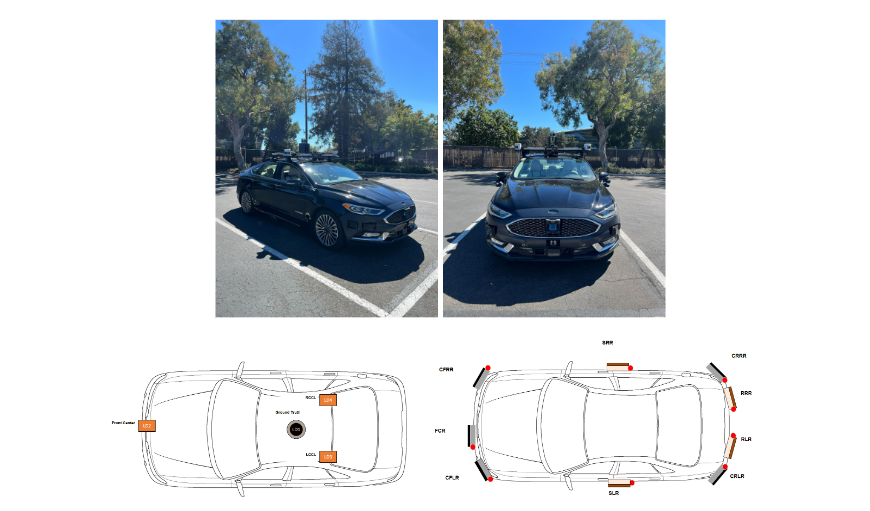
Vehicle setup
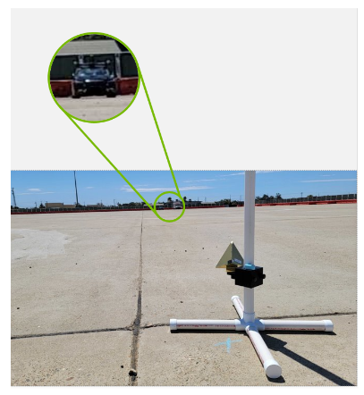
We used radar sensors in the NVIDIA DRIVE Hyperion AV reference architecture, so developers building on NVIDIA DRIVE can easily transition between simulation and the real world. The sensors were mounted on a development vehicle (Figure 3). For this case, the front center radar (FCR) was the focus for evaluation.
Operating at a frequency of 77GHz, the radar under test included two scans: a near scan, with a wide FOV but limited range, and a far scan with extended range but a narrow FOV. Additionally, a 360° rotating lidar sensor (LD1) was mounted on top of the car to provide pseudo ground truth data.
Model validation process
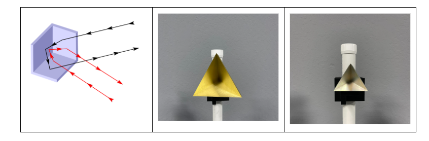
Central to our three validation experiments were two trihedral corner reflectors. These are standard radar targets that reflect energy back in the incident direction. They are characterized by a radar cross-section (RCS) value, which is a measure of an object’s ability to reflect radar energy back to the receiver.
We used one with a “high” RCS of 15.71 decibels relative to a square meter (dBsm), and another with a “low” RCS of 4.79 dBsm to characterize the model’s behavior across a wide RCS range.
The lidar’s pseudo-ground truth measurements were used to replicate the test setup virtually in DRIVE Sim with accurate material assignments.
After collecting the virtual data, we compared the radar model outputs to the real radar. Results of the comparison are presented for the three scenarios below.
Scenario 1: FOV sampling with corner reflector
In the first scenario, we assessed the radar’s detection capabilities across its FOV and verified its range and azimuth accuracy.
We placed a corner reflector at multiple grid positions within the radar’s FOV, as shown in Figure 5. We assumed the sensor’s behavior to be symmetric, and thus we only sampled half of the FOV to increase the sampling density.
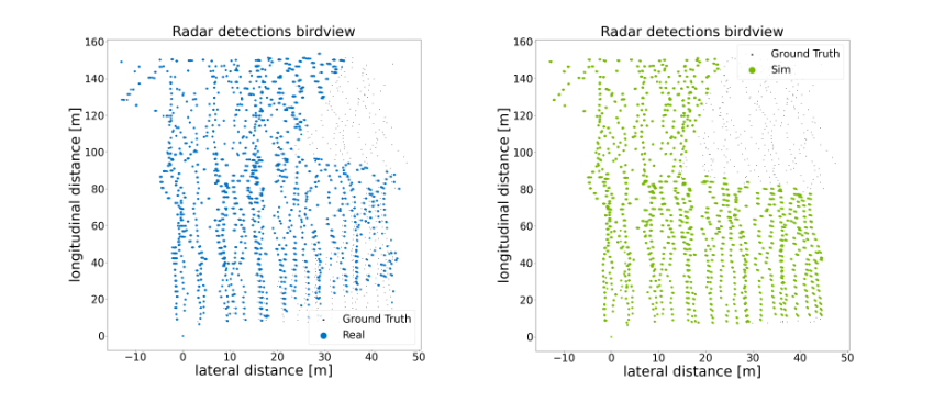
Altogether, we recorded a total of 579 positions for the high RCS corner reflector and 632 for the low RCS corner reflector.
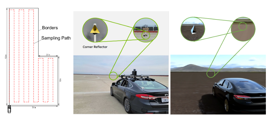
Figure 6 depicts a top-down view of both real and simulated radar detections across all 1,211 high and low RCS corner reflector positions. We used this as a coherence check to start. Although we observed differences in FOV coverages above 80m, the overall coverage presented a noticeable similarity that is sufficient for the cross check.
The histograms in Figure 7 present the error distribution in range, azimuth, and RCS relative to the ground truth for both the high and low RCS corner reflectors, combined. Where applicable, we quantified the results by fitting a Gaussian distribution to the data. Results for the real radar are displayed on the left, while the DRIVE Sim data is shown on the right.
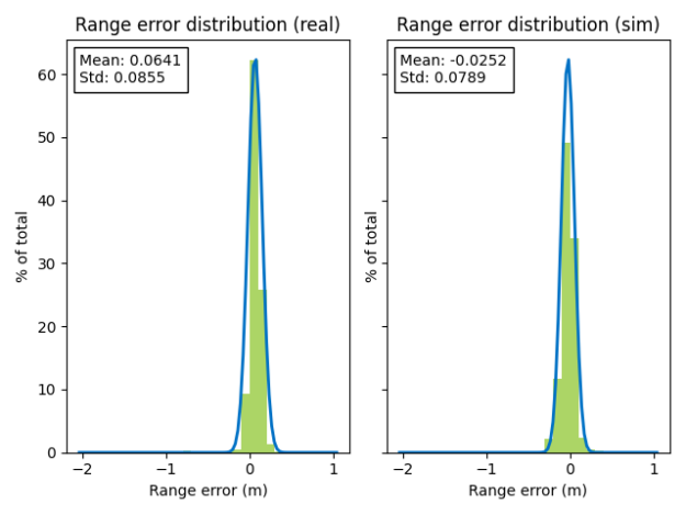
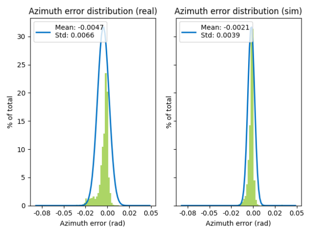
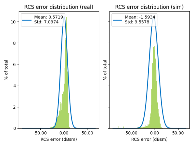
We observed a high level of agreement between real and simulation data over various positions in the radar’s FOV, with both means and standard deviations sharing the same order of magnitude.
The discrepancies are primarily attributable to uncertainties in the ground truth. While the lidar sensor has millimeter-level accuracy, identifying the position and orientation of an object like a pole-mounted corner reflector can introduce errors in the centimeter range. Furthermore, while we calibrated the sensor positions prior to data collection, there might still be minor misalignments.
Overall, the agreement observed in RCS values, detection pattern, and the accuracies of the various detection properties validated the radar’s fidelity, wave propagation, and material modeling.
Scenario 2: Corner reflector separation capability test
In scenarios where road objects are near each other (stationary vehicles under a bridge, pedestrians or motorcyclists next to a vehicle or guard rail, or two closely parked cars, for example) radars can encounter difficulties in distinguishing individual objects. For this reason, it is crucial to accurately simulate this characteristic, known as separation capability.
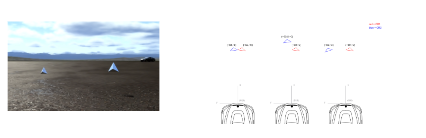
We assessed this capability by placing the two corner reflectors in close proximity to each other. The data was sampled at four different distances from the sensor. For each distance, the corner reflectors were positioned as shown in Figure 8.
We selected different positions for the radar’s near and far scans, dependent on their corresponding FOV, to analyze their range and azimuth separation capabilities.
Tables 1 and 2 summarize the results for the near and far scans. The left column represents positions where CRs are close and we expect one detection per the TPS. The center and right columns represent positions where we expect two detections per the TPS. Each cell details the exact location of the CRs, and the number of detections observed for simulation and the real world. The percentage denotes the proportion of detections that followed our expectations in all considered scans. We define success when the simulated and real percentages are less than 20% apart.
| Position of CRs (x,y) in meters | Position of CRs (x,y) in meters | Position of CRs (x,y) in meters | |
| 0° and 50m | CR1 (50, 0), CR2 = CR1 Real: One detection (100%) Sim: One detection (100%) | CR1 (50, 0), CR2 (50.5, 0) Real: Two detections (10%) Sim: Two detections (0%) | CR1 (50, 0), CR2 (50, -3) Real: Two detections (0%) Sim: Two detections (0%) |
| -45° and 20m | CR1 (14.14, -14.14), CR2 = CR1 Real: One detection (100%) Sim: One detection (100%) | CR1 (14.14, -14.14),CR2 (15.14, -14.14) Real: Two detections (100%) Sim: Two detections (100%) | CR1 (14.14, -14.14), CR2 (16.44, -11.84) Real: Two detections (100%) Sim: Two detections (100%) |
| -45° and 50m | CR1 (35.36, -35.36), CR2 = CR1 Real: One detection (100%) Sim: One detection (100%) | CR1 (35.36, -35.36),CR2 (36.36, -35.36) Real: Two detections (5%) Sim: Two detections (100%) | CR1 (35.36, -35.36), CR2 (41, -29) Real: Two detections (80%) Sim: Two detections (100%) |
Results for all positions at 0° and 50m, and -45° and 20m, demonstrated a high degree of similarity between real and simulated. We observed a minor discrepancy at 0° and 50m where CR2 (50.5, 0). In this scenario, the real radar returned two detections instead of one in 10% of the scans.
Comparisons made at -45° and 50m were mostly consistent, except for CR2 (36.36, -35.36), where the simulated radar returned two detections.
| Position of CRs (x,y) in meters | Position of CRs (x,y) in meters | Position of CRs (x,y) in meters | |
| 0° and 50m | CR1 (50, 0), CR2 = CR1 Real: One detection (100%) Sim: One detection (95%) | CR1 (50, 0), CR2 (50.5, 0) Real: One detection (100%) Sim: One detection (5%) | CR1 (50, 0), CR2 (50, -3) Real: Two detections (0%) Sim: Two detections (5%) |
| 0° and 100m | CR1 (100,0), CR2 = CR1 Real: One detection (100%) Sim: One detection (60%) | CR1 (100, 0), CR2 (104, 0) Real: Two detections (100%) Sim: Two detections (95%) | CR1 (100, 0), CR2 (100, -6) Real: Two detections (0%) Sim: Two detections (0%) |
As shown in Table 2, the results from the simulated and real-world sensors are largely in correlation. Significant deviations are noted at 0° and 50m where CR2 (50.5, 0). Furthermore, for 0° and 100m where CR1=CR2, the simulated radar returns two detections in 40% of scans, while real world never returns two detections.
Upon further analysis of the deviations, we attribute them to the fact that the technical product specification only described the radar’s separation capability at a few angles. This made it difficult for us to estimate the exact layout of range and azimuth bins.
In addition, our parameterization and implementation for the CFAR thresholding algorithm is an estimate, as it is a supplier’s intellectual property. The separation capability of the radar is expected to be quite sensitive to the CFAR behavior.
Overall, across both the near and far scans, we found the simulated separation capability to be close enough to the real sensor.
Scenario 3: Driving toward a corner reflector with constant speed
Doppler measurement enables radars to accurately detect the speed of moving targets. We evaluated the model’s performance in dynamic conditions, where the test vehicle drove directly toward high and low RCS corner reflectors, taking separate trips at constant speeds of 10kph, 40kph, and 80kph, as shown below.
The histograms in Figure 11 present the Doppler error results for both the high and low RCS corner reflectors.
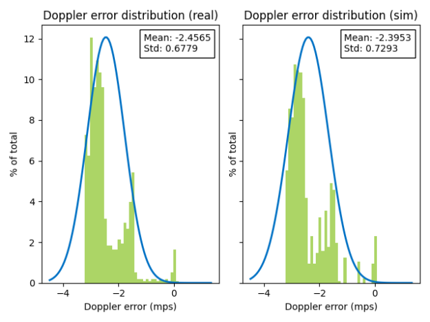
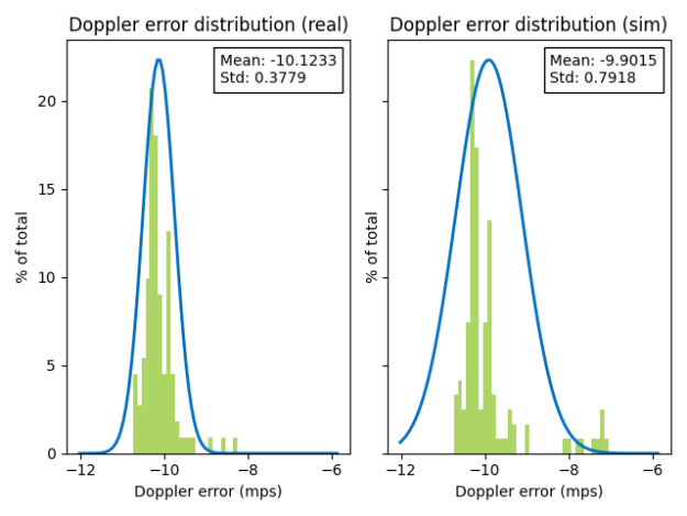
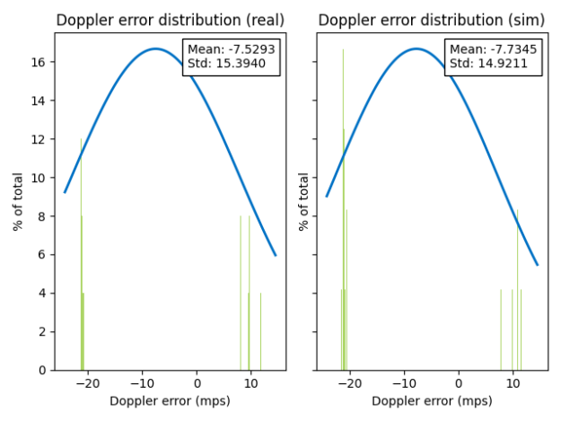
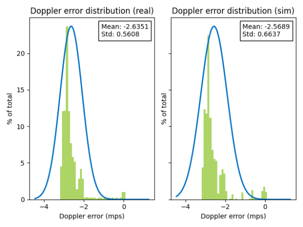
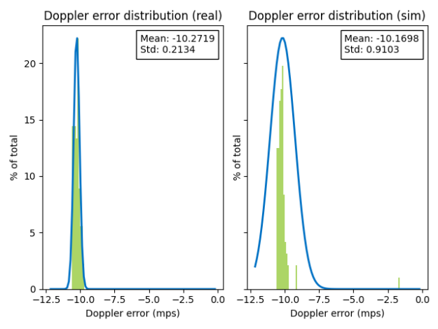
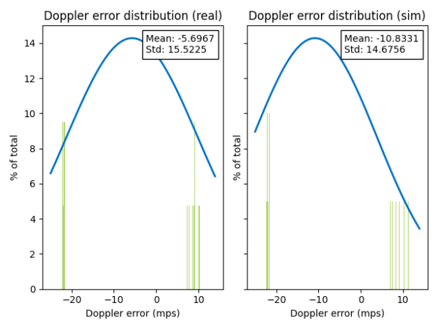
Figure 11. Doppler error histograms for Scenario 3
We observed a remarkably high correlation in Doppler across all tested speeds. For 10kph, both real and simulated distributions exhibited similar peaks at approximately -3mps, -2mps, and 0mps. For 40kph, the peaks aligned around -10mps. For 80kph, peaks were observed at -20mps and 10mps. This high degree of accuracy was further demonstrated when plotting Doppler against range.
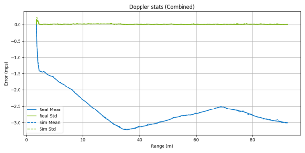
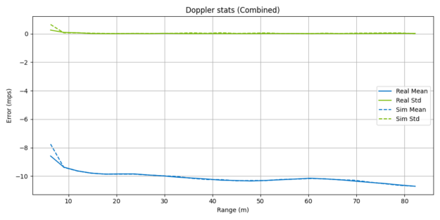
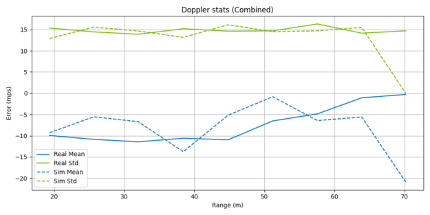
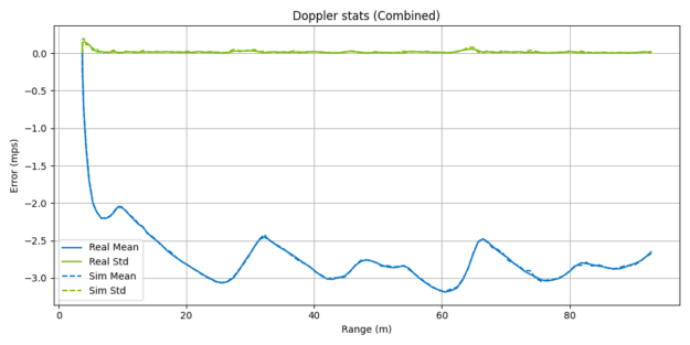
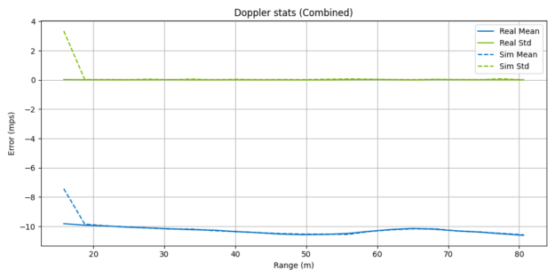
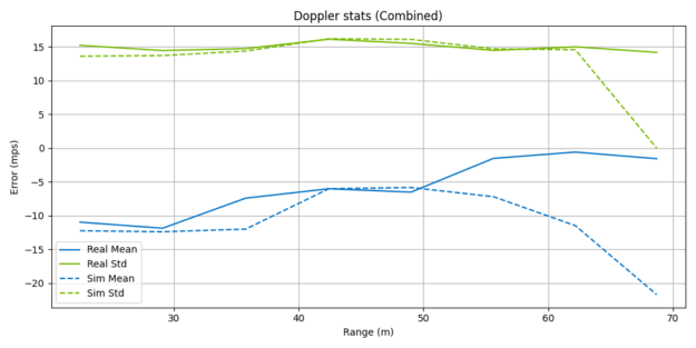
Figure 12. Doppler mean eror and standard deviation over the range for Scenario 3
Figure 13 illustrates a top-down view of real and simulated radar detections across high and low RCS corner reflector positions and vehicle speeds.
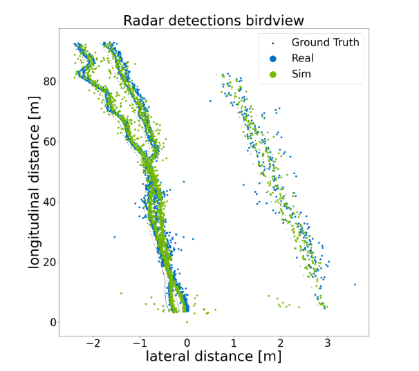
Both the real and simulated Doppler measurements demonstrated substantial agreement in their mean and standard deviation values. However, we noticed deviations at higher speeds.
We attribute these deviations to uncertainties during the creation of the digital twin. The position, speed, and orientation of the ego vehicle were estimated using lidar without the aid of differential GPS. The errors in these estimations are amplified at higher speeds as can be seen in 80kph.
In addition, we observed that DRIVE Sim is able to replicate the Radar Aliasing phenomenon, which occurs when an object’s radial velocity surpasses the radar’s maximum measurable unambiguous velocity, resulting in ambiguous velocity values. Real-world radars subtly shift the maximum measurable unambiguous velocity range with each cycle, enabling subsequent perception algorithms to disambiguate the velocities.
Our simulation accurately replicated this behavior, as demonstrated by the alignment of the peaks in both the real and simulated data. Particularly, at a speed of 80kph, both the real and simulated radar exhibited similar velocity wrapping.
Conclusion
This study presents our first iteration for an in-depth validation of our simulated radar model using real-world data, including static and dynamic conditions. The analysis was designed to assess the model’s fidelity and accuracy across a variety of performance metrics.
Our results demonstrate a high degree of correlation between the simulated and real-world radar data with the model adeptly handling complex interactions such as multibounce effects.
Upcoming experiments will focus on capturing radar data from more complex objects (vehicles, pedestrians, motorbikes) mimicking real-world scenarios. These objects not only have more complicated geometries, but are also composed of a variety of materials, thus introducing further complexities in radar wave interactions. Through these efforts, we aim to continually enhance the model’s fidelity, further bridging the gap between simulation and reality.
By validating accurate radar sensor behavior in simulated scenarios, we can improve system development efficiency, reduce dependence on costly and time-consuming real-world data collection, and enhance the safety and performance of AV systems.
To learn more, see our previously published posts:
