NVIDIA Riva is an application framework that provides several pipelines for accomplishing conversational AI tasks. Generating high-quality, natural-sounding speech from text with low latency, also known as text-to-speech (TTS), can be one of the most computationally challenging of those tasks.
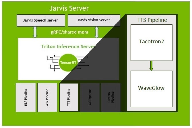
In this post, we focus on optimizations made to a TTS pipeline in Riva, as shown in Figure 1. For more information about the Riva Server, see Introducing NVIDIA Riva: A GPU-Accelerated SDK for Developing Speech AI Applications.
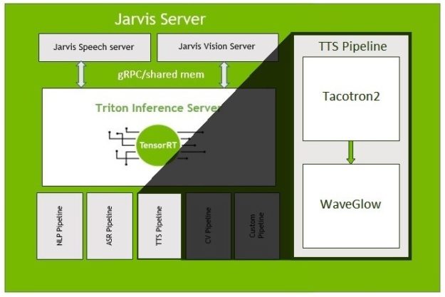
This TTS model is composed of the Tacotron2 network, which maps character sequences to mel-scale spectrograms, followed by the NVIDIA WaveGlow network, which generates time-domain waveforms from the mel-scale spectrograms. For more information about the networks, as well as how to train them using PyTorch, see Generate Natural Sounding Speech from Text in Real-Time.
Our goal in creating the Riva TTS pipeline was to enable conversational AIs to respond with natural-sounding speech in as little time as possible, making for an engaging user experience. Below, we detail the effort of creating a high-performance, TTS, inference implementation, using NVIDIA TensorRT and CUDA.
In a previous post, How to Deploy Real-Time Text-to-Speech Applications on GPUs using TensorRT, you learned how to import a TTS model from PyTorch into TensorRT, to perform faster inference with minimal effort.
For this implementation, we wanted to get the lowest latency TTS inference that we could. To accomplish this, we made several decisions, that while they require more effort, result in additional performance. The implementation discussed in this post is available as part of the NVIDIA Deep Learning Examples GitHub repository.
Creating the networks in TensorRT
To start with, we used the C++ TensorRT interface rather than the Python bindings. This helped to reduce the amount of overhead time needed on the CPU to coordinate and launch work on the GPU. For more information about creating and running networks with the C++ API, see Using the C++ API.
This is particularly important in Tacotron2, where we must launch a network execution to generate each mel-scale spectrogram frame, of which there are roughly 86 per second of audio.
Creating Tacotron2 using IBuilder
To gain more flexibility in the Tacotron2 network, instead of parsing the exported ONNX model and having TensorRT automatically create the network, we manually constructed the network through the IBuilder interface of TensorRT. This enabled us to make several modifications, including allowing variable-length sequences in the same batch to be processed.
To build the network manually, we first needed an easy way to get the weights from PyTorch to C++. For ease of use and readability, we used a single-level JSON structure. Another option would be to get the weights using the PyTorch C++ API. To export the Tacotron2 PyTorch model to JSON, use the following command:
statedict = dict(torch.load(statedict_path)["state_dict"])

outdict = {}

for k, v in dict(statedict).items():

    if k.startswith("module."):

        k = k[len("module."):]

    outdict[k] = v.cpu().numpy().tolist()

with open(json_path, "w") as fout:

    json.dump(outdict, fout)
To get the weights into a format that the TensorRT C++ API can consume, we created the JSONModelImporter and LayerData classes, which handle reading and storing the weights as Weights. These can be passed into TensorRT layers.
As in the ONNX-parsed implementation of Tacotron2, we split it up into three subnetworks: the encoder, decoder, and post-net, which we created with the EncoderBuilder, DecoderPlainBuilder, and PostNetBuilder classes, respectively.
At the start of the build methods, we created the INetworkDefinition object from IBuilder, and also added inputs.
Encoder network
The encoder network consists of an embedding layer, followed by convolution layers with activations, and ends with a bidirectional LSTM. Because the encoder is only run one time during inference, it tends to take a small fraction of the runtime, less than five percent in most cases.
While the bidirectional LSTM in TensorRT allows setting individual sequence lengths in batches, we needed to prevent the padding from impacting the convolution layers. To do this, we added a second input of a mask vector, which is all ones for the length of the sequence, followed by all zeros for the length of the padding. Then, on the output of each convolution layer, an element-wise multiplication with this mask is performed to reset the padding to zeros of each item in the batch.
Decoder network
The decoder network is run one time for every mel-scale spectrogram frame produced, which in this configuration is roughly 86 times for every second of output audio until the stop condition is met. It is by far the most expensive part of the Tacotron2 network. It consists of a prenet, location-sensitive attention (LSA), and LSTM cells, and ends with projection layers.
To amortize the cost of synchronously copying the stop token value back to the CPU, a fixed number of decoder iterations are run before reading the value of the accumulated stop tokens. This amortizes the cost of synchronously copying data from GPU to CPU over a larger amount of work.
All of the random numbers needed for the dropouts in the prenet are generated at the start of each group of decoder iterations. Generating many random numbers at one time is more efficient than repeatedly generating few random numbers in separate kernels.
The LSA is the only part of the decoder network that makes use of the padded input. As such, the same mask vector from the encoder is re-used to reset that padding to zero after the convolution layer. The TensorRT IRaggedSoftMaxLayer layer, allows the soft-max to be performed on variable sequence lengths within a batch.
We merged the two fully connected layers at the end of the network, the 80×1536 layer for generating the mel-scale spectrogram frame and the 1×1536 layer for creating the stop token, into a single 81×1536 layer. This helps to increase parallelism and reduce the number of kernels launched.
Post-net network
The post-net network consists of five convolution layers followed by activations. To get good performance out of it, we input a fixed number of mel-spectrograms, to allow TensorRT to choose the optimal configuration with which to run it. In this configuration, the post-net network tends to take a small fraction of the runtime, less than five percent in most cases.
Creating WaveGlow using the ONNX parser
Unlike Tacotron2, WaveGlow does not need any internal modification to work properly on variable-length sequences when using batching. For this portion of our speech pipeline, we followed the nominal PyTorch to ONNX and ONNX to TensorRT path. To export the model, we used torch.onnx.export and marked the batch dimension as dynamic.
torch.onnx.export(model, (mels, z),
                  output_path,
                  dynamic_axes={'mels': {0: 'batch_size'},
                                'audio': {0: 'batch_size'}},
                  input_names=['mels', 'z'],
                  output_names=['audio'],
                  opset_version=10)
Because the potential input/output length for the WaveGlow network is highly variable, from several dozen mel-scale spectrograms to hundreds, we use a static dimension for the input/output length of two seconds and cut the output down to the appropriate size for shorter chunks. This enables TensorRT to optimize for a specific size while enabling us to process the variable-length sequences encountered in TTS.
We did not specify ‘z’ as having a dynamic batch size. Because we are only doing inference, we broadcast the same random ‘z’ across all items in the batch but generate a new ‘z’ for each chunk.
Optimizing performance further
We used NVIDIA Nsight Systems to gain more detailed insight into how our TTS implementation is using the hardware. Figures 2 and 3 show the GPU utilization profiles of Tacotron2 and WaveGlow, respectively.


We can see that this Tacotron2 implementation is CPU-bound, letting the GPU go idle in between its many small kernel launches. This is because many of the kernels take just a few microseconds to complete, and the CPU cannot generate work fast enough for the GPU.
WaveGlow on the other hand, with its larger kernels, gets good utilization out of the GPU, and the CPU can generate work fast enough to keep the GPU busy.
Using custom plugins for the Tacotron2 decoder loop
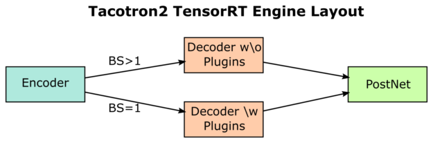
The low utilization of the GPU in Tacotron2 begins to fade away when the batch size is increased and with it, the amount of work per kernel. The many bandwidth-bound general matrix-vector (GeMV)-like operations become more compute-heavy, general matrix multiply (GeMM)-like operations. This meant that we could focus performance improvements on the batch size of one case, which is common in TTS applications.
To achieve maximum performance in the Tacotron2 network, we replaced many of the small layers in the decoder with custom layers, using the TensorRT IPluginV2DynamicExt interface. This gave us the ability to perform several low-level optimizations, while still letting TensorRT do the heavy lifting for other parts of our network. We built the decoder network with plugins in the DecoderBuilderPlugins class.
We split the decoder iteration into four separate plugins:
- Prenet
- LSTM cell
- Attention
- Projection
We changed our C++ backend, to switch between the decoder without plugins for batch sizes greater than one, and our decoder with plugins for a batch size of one, as shown in Figure 5.
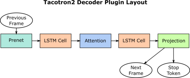
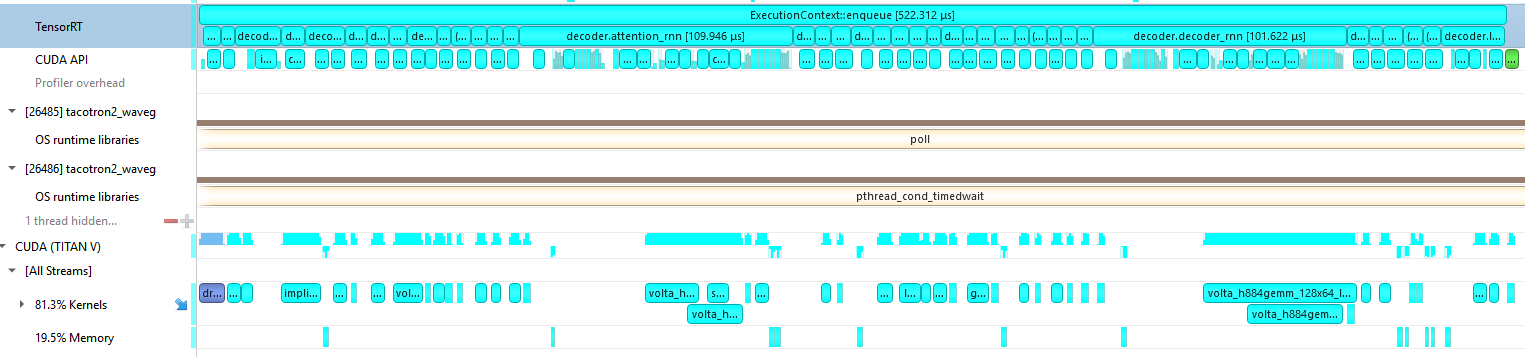
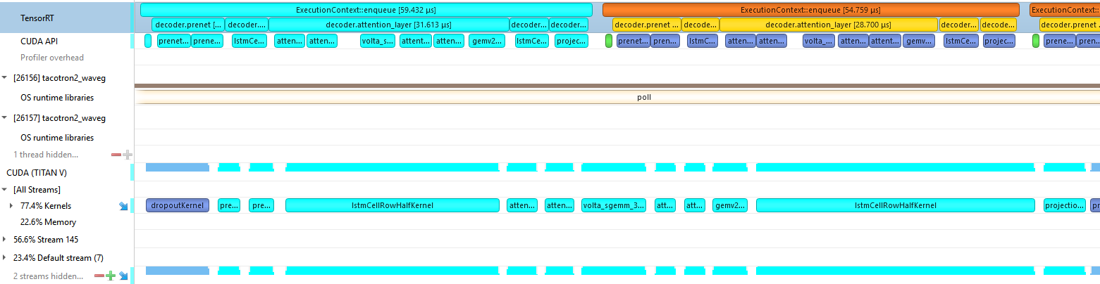
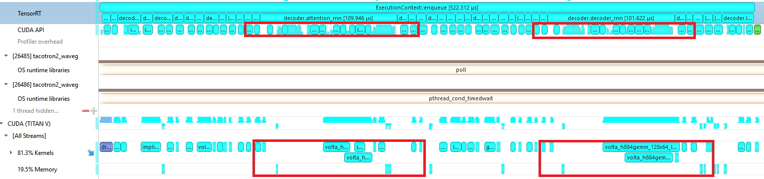
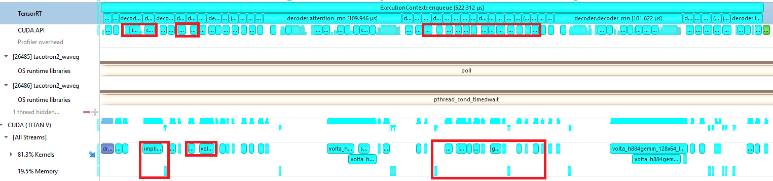
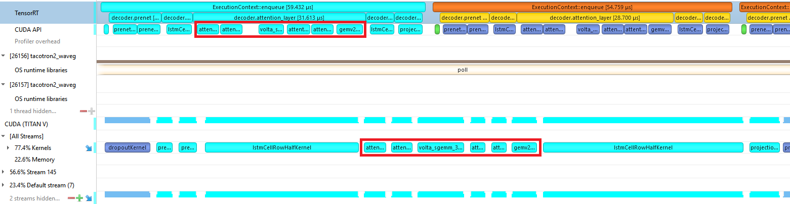
Figure 6 shows the profile of a Tacotron2 decoder iteration before we implemented any custom plugins. The CPU work required to launch many little kernels is the bottleneck, and you can see many gaps in GPU work at the bottom.
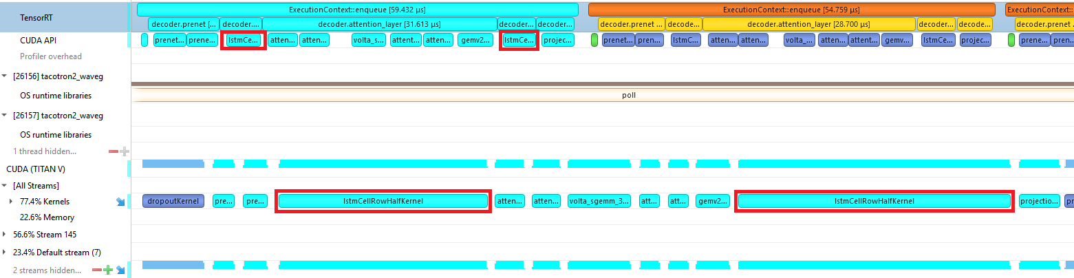
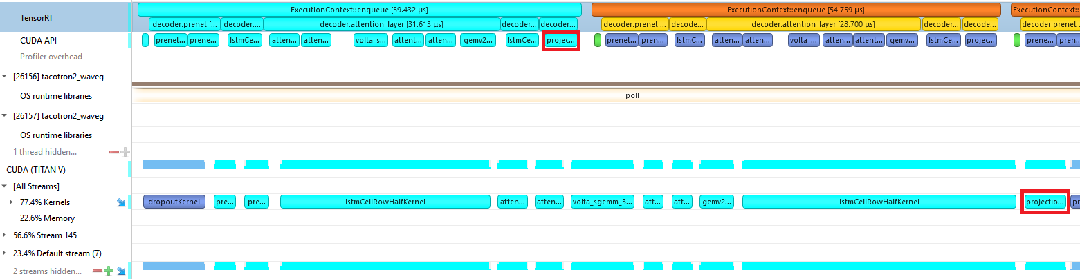
Figure 7 shows the profile of a Tacotron2 decoder iteration using the custom plugins. The CPU is only working on launching kernels for the iteration for half of the time that it takes the GPU to run them. This keeps the GPU busy and enables the CPU to move on to queuing up work for the next iterations.
Our work in fusing kernels and reducing CPU overhead led to nearly a 10x reduction in the CPU time required to launch an iteration and a 5x reduction in GPU time. Because these custom layers are specific to our network, we were able to do low-level CUDA optimizations. This includes using template parameters as layer dimensions, which lets the compiler perform aggressive optimizations, as well as avoiding bounds checking by using block sizes which are a multiple of the weight dimensions.
Prenet plugin
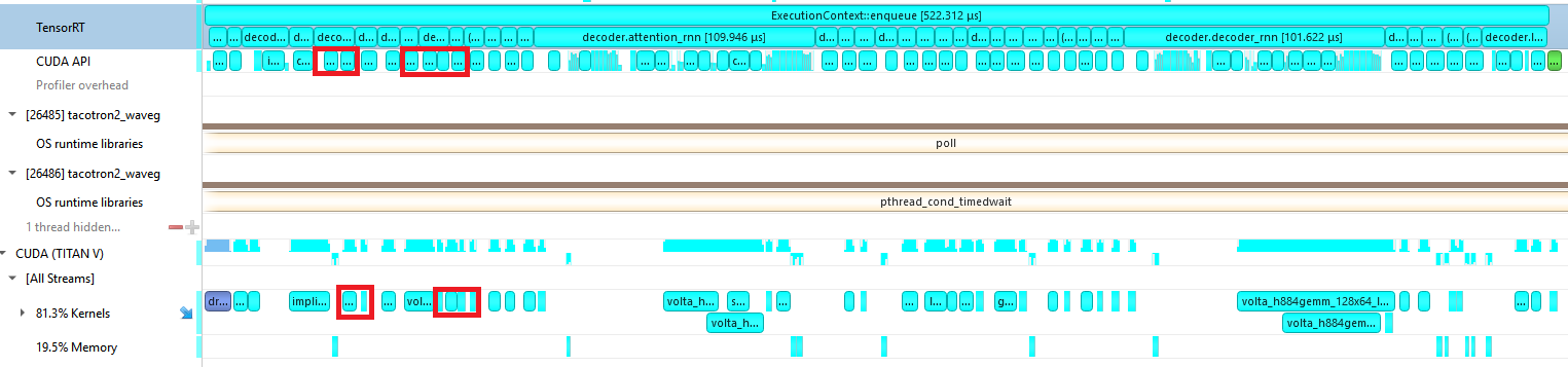
Originally, the two layers of the prenet were implemented as a fully connected layer, followed by an element-wise multiplication against random vectors of 0 and (1/1-p) to emulate the dropout, and finally a rectified linear unit (ReLU) activation. This resulted in three kernels per layer, as can be seen in Figure 8.
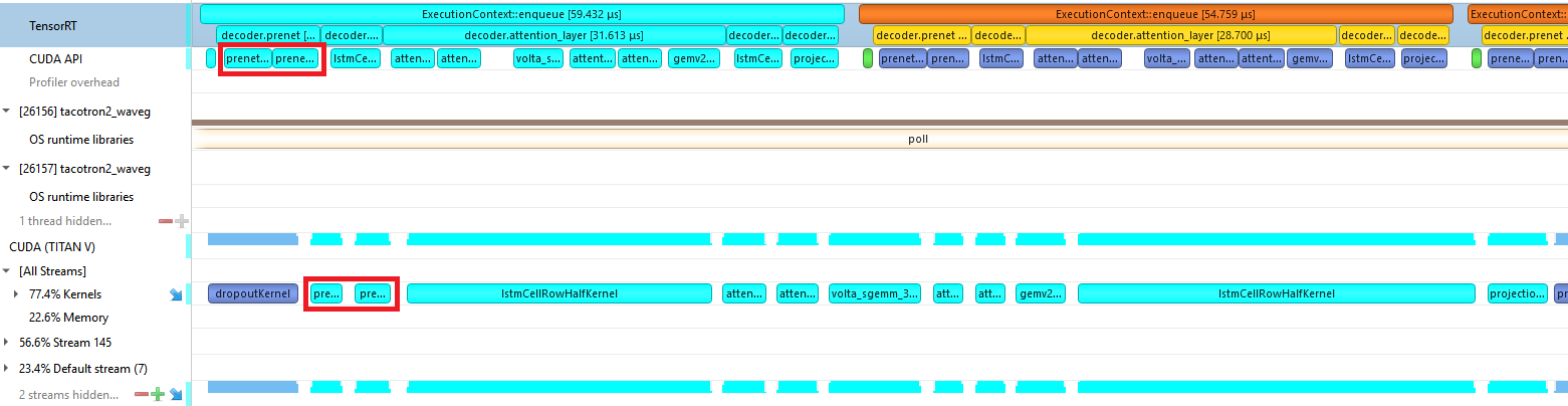
The plugin for the prenet uses a CUDA kernel that fuses the fully connected layer with the dropout and subsequent ReLU. It is implemented in the file src/trt/plugin/taco2PrenetPlugin/taco2PrenetKernel.cu. We call this kernel twice to handle both layers in the prenet. This reduces six kernel calls to two, as seen in Figure 9.
LSTM cell plugin
The plugin for the LSTM cells fuses a concat operation on the input with the LSTM cell computation. Our LSTM cell kernel is implemented in the file src/trt/plugin/taco2LSTMCellPlugin/taco2LSTMCellKernel.cu.
While the NVIDIA CUDA Deep Neural Network library (CUDNN) implementation, which creates new streams and launches GeMVs on each stream to maximize parallelism, works well for LSTMs with a sequence length greater than one, the overhead for stream creation and multiple kernel launches do not amortize well enough for our purposes (Figure 10).
As such, our custom kernel loads the two separate inputs, performs both GeMVs, adds both biases, and computes the hidden and cell states. Doing this all in one kernel also reduces the amount of reads and writes that we need to make to global memory.
To avoid being memory-bound when loading the weights from global memory, we store the weights as FP16 but still perform the computation in FP32 to preserve accuracy enough for the LSA. Figure 11 shows the effects of these optimizations, where we have a single kernel per LSTM cell.
Attention plugin
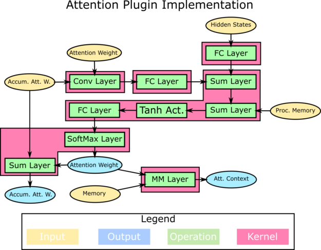
The Attention plugin is the most complex of the four plugins, making use of six CUDA kernels. Figure 13 shows the division of the operations into those CUDA kernels.
We made use of the high-performance NVIDIA cuBLAS library GeMV and GeMM implementations for the FC and MM layers. For the convolution layer, we used a custom CUDA kernel that had the number of channels and kernel size hard-coded for the Tacotron2 network.
We fused the first set of element-wise sums and activation with the FC layer before the SoftMax. Then, we fused the SoftMax with the element-wise summation required for the accumulation of the Attention weights.
Figure 14 shows the result of the work on this plugin, where launching the six kernels takes only 29 microseconds.
Projection plugin
The projection plugin is relatively simple, fusing a concatenation with a fully connected layer. Because this layer has only 81 rows in the weight matrix, we used one row per thread block, to ensure the kernel could occupy as many SMs as possible, and thus make the most use of the available memory bandwidth when loading the weights.
Figure 15 shows the concatenation and projection used to require several memory operations and kernel launches (the GeMV plus some reformatting). In our plugin, this is now reduced to a single kernel, as shown in Figure 16.


Demonstrating end-to-end performance
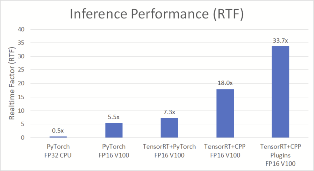
Figures 17 and 18 compare the end-to-end inference performance of the Tacotron2 and WaveGlow TTS pipeline. Latency is measured from the start of Tacotron2 to the end of WaveGlow. All implementations were given the same 128-character input sequence and generated between 6.4 and 7.0 seconds of audio.
The variation in output length is due to the random dropouts in the prenet, and small numerical differences in the implementations affecting the LSA. The PyTorch FP32 CPU run was generated on an Intel Xeon E5-2698 v4, and then others were generated on an NVIDIA V100 GPU.

The implementation using the TensorRT C++ API with plugins for the decoder loop (TRT+CPP Plugins), delivers 6.7 seconds of audio in 200 ms. We made use of the TensorRT performance-critical features and better use of the power of the GPU.
In Figure 18, the real-time factor (RTF) is the latency divided by the wall clock time, the number of seconds of audio generated per second. An implementation with an RTF of 1.0 generates audio in real time. On the V100 using TensorRT 7.0, this optimized implementation achieved 33.7x faster than real-time, end-to-end, TTS inference.
New A100 GPU and TensorRT 7.1
With the newly announced NVIDIA A100 GPU and TensorRT 7.1, the performance of the TTS pipeline gets even better.
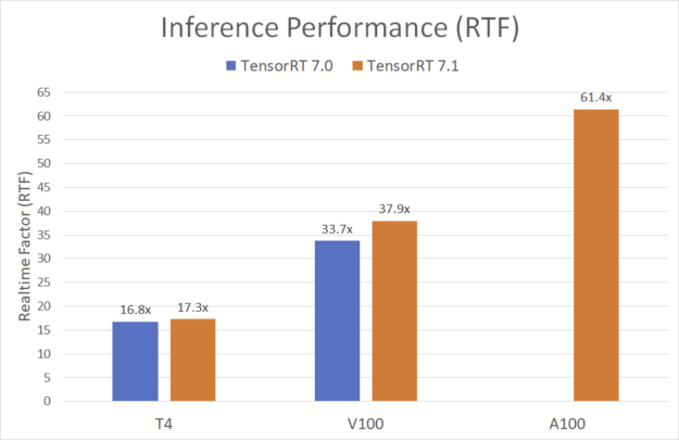
Figure 19 shows that, on A100 with TensorRT 7.1, the TTS pipeline achieves a blisteringly fast 61.4x RTF, generating 7.3 seconds of natural-sounding speech in less than 120 milliseconds. This high-performance speech synthesis is a crucial component of conversational AI, giving users immediate answers to their questions and creating a truly engaging experience. The performance improvements made in TensorRT 7.1 further improve the performance on the NVIDIA T4 GPU and V100 platforms.
Running the TTS pipeline
This standalone TTS pipeline is available as part of the NVIDIA Deep Learning Examples repository. You can check it out and run it yourself with the following instructions.
Clone the repository
First, clone the NVIDIA Deep Learning Examples repository, and navigate to the Tacotron2 C++ directory:
git clone https://github.com/NVIDIA/DeepLearningExamples
cd DeepLearningExamples/PyTorch/SpeechSynthesis/Tacotron2/trtis_cpp
Export the models
You can either train models yourself or download pretrained checkpoints from NVIDIA NGC and copy them to the ./checkpoints directory:
mkdir checkpoints
cp <Tacotron2_checkpoint> ./checkpoints/
cp <WaveGlow_checkpoint> ./checkpoints/
Next, export the PyTorch checkpoints so that they can be used to build TensorRT engines. This can be done using the script export_weights.sh script:
mkdir models
./export_weights.sh checkpoints/tacotron2_1032590_6000_amp checkpoints/waveglow_1076430_14000_amp models/
Set up the Triton server
To build the Docker container for the Triton server, run the build_trtis.sh script:
./build_trtis.sh models/tacotron2.json models/waveglow.onnx models/denoiser.json
This takes some time as TensorRT tries out different tactics for best performance while building the engines.
Set up the Triton client
Next, build the client Docker container. To do this, enter the trtis_client directory and run the script build_trtis_client.sh:
cd trtis_client
./build_trtis_client.sh
cd ..
Run the Triton server
To run the server locally, use the script run_trtis_server.sh:
./run_trtis_server.sh
To set which GPUs the Triton server sees, use the environment variable NVIDIA_VISIBLE_DEVICES.
Run the Triton client
Leave the server running. In another terminal window, type:
cd trtis_client/
./run_trtis_client.sh phrases.txt
This generates one WAV file per line in the file phrases.txt, named after the line number (for example, 1.wav through 8.wav for an 8-line file) in the audio/ directory. It is important that each line in the file ends with a period, or Tacotron2 may fail to detect the end of the phrase.
