Sign up for the latest Speech AI News from NVIDIA.
This post, intended for developers with professional level understanding of deep learning, will help you produce a production-ready, AI, text-to-speech model.
Converting text into high quality, natural-sounding speech in real time has been a challenging conversational AI task for decades. State-of-the-art speech synthesis models are based on parametric neural networks1. Text-to-speech (TTS) synthesis is typically done in two steps.
- First step transforms the text into time-aligned features, such as mel spectrogram, or F0 frequencies and other linguistic features;
- Second step converts the time-aligned features into audio.
The optimized Tacotron2 model2 and the new WaveGlow model1 take advantage of Tensor Cores on NVIDIA Volta and Turing GPUs to convert text into high quality natural sounding speech in real-time. The generated audio has a clear human-like voice without background noise.
Here is an example of what you can achieve using this model:
Input:
“William Shakespeare was an English poet, playwright and actor, widely regarded as the greatest writer in the English language and the world’s greatest dramatist. He is often called England’s national poet and the ‘Bard of Avon’.”
Output:
After following the steps in the Jupyter notebook, you will be able to provide English text to the model and it will generate an audio output file. All of the scripts to reproduce the results have been published on GitHub in our NVIDIA Deep Learning Examples repository, which contains several high-performance training recipes that use Tensor Cores. Additionally, we developed a Jupyter notebook for users to create their own container image, then download the dataset and reproduce the training and inference results step-by-step.
The Models
Our TTS system is a combination of two neural network models:
- A modified Tacotron 2 (Figure 1) model from the “Natural TTS Synthesis by Conditioning WaveNet on Mel Spectrogram Predictions” and;
- A flow-based neural network model from the “WaveGlow: A Flow-based Generative Network for Speech Synthesis”.
The Tacotron 2 and WaveGlow model form a TTS system that enables users to synthesize natural sounding speech from raw transcripts without any additional prosody information.
Tacotron 2 Model
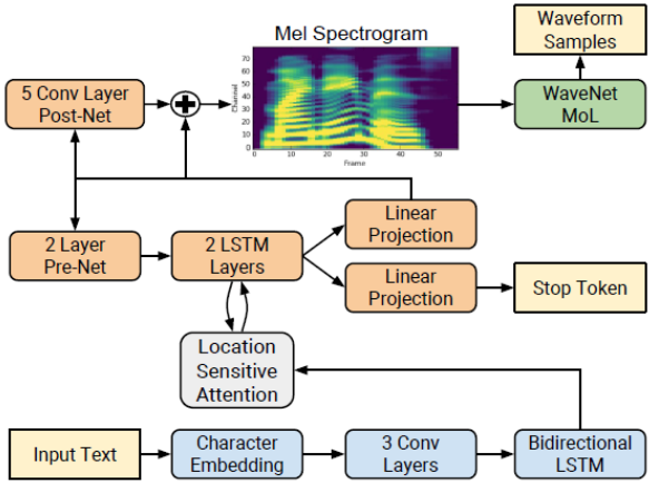
Tacotron 22 is a neural network architecture for speech synthesis directly from text. The system is composed of a recurrent sequence-to-sequence feature prediction network that maps character embeddings to mel-scale spectrograms, followed by a modified WaveNet model acting as a vocoder to synthesize time-domain waveforms from those spectrograms, as shown in Figure 1.

The network is composed of an encoder (blue) and a decoder (orange) with attention. The encoder converts a character sequence into a hidden feature representation, which serves as input to the decoder to predict a spectrogram. Input text (yellow) is presented using a learnt 512-dimensional character embedding, which are passed through a stack of three convolutional layers (each containing 512 filters with shape 5 × 1), followed by batch normalization and ReLU activations. The encoder output is passed to an attention network (gray) which summarizes the full encoded sequence as a fixed-length context vector for each decoder output step.
The decoder is an autoregressive recurrent neural network which predicts a mel spectrogram from the encoded input sequence one frame at a time. The prediction from the previous timestep is first passed through a small pre-net containing two fully connected layers of 256 hidden ReLU units. The prenet output and attention context vector are concatenated and passed to a stack of two LSTM layers with 1,024 units. The concatenation of the LSTM output and the attention context vector is projected through a linear transform to predict the target spectrogram frame. Finally, the predicted mel spectrogram is passed through a 5-layer convolutional post-net which predicts a residual to add to the prediction to improve the overall reconstruction. Each post-net layer is comprised of 512 filters with shape 5 × 1 with batch normalization, followed by tanh activations on all but the final layer.
Our implementation of the Tacotron 2 model differs from the model described in1, we use:
- Dropout instead of Zoneout to regularize the LSTM layers;
- WaveGlow model2 instead of WaveNet to synthesize waveforms.
WaveGlow Model
WaveGlow 1 is a flow-based network capable of generating high-quality speech from mel spectrograms. WaveGlow combines insights from Glow5 and WaveNet6 in order to provide fast, efficient and high-quality audio synthesis, without the need for auto-regression. WaveGlow is implemented using only a single network, trained with only a single cost function: making the training procedure simple and stable. Our current model synthesizes samples at 55 * 22,050 = 1,212,750, which is 55 times faster than “real-time” at 22,050 samples per second sampling rate. The Mean Opinion Score (MOS) show that it delivers audio quality as good as the best publicly available WaveNet implementation trained on the same dataset.
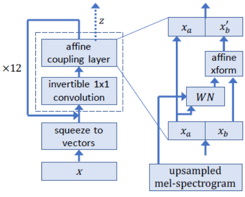
WaveGlow is a generative model that generates audio by sampling from a distribution. To use a neural network as a generative model, we take samples from a simple distribution, in our case, a zero mean spherical Gaussian with the same number of dimensions as our desired output, and put those samples through a series of layers that transforms the simple distribution to one which has the desired distribution. In this case, we model the distribution of audio samples conditioned on a mel spectrogram.
As depicted in Figure 2, for the forward pass through the network, we take groups of eight audio samples as vectors, the ”squeeze” operation, as in Glow5. We then process these vectors through several ”steps of flow”. A step of flow here consists of an invertible 1 × 1 convolution followed by an affine coupling layer. Within the affine coupling layer, half of the channels serve as inputs, which then produce multiplicative and additive terms that are used to scale and translate the remaining channels.
Enable Automatic Mixed Precision
Mixed precision training offers significant computational speedup by performing operations in half-precision format, while storing minimal information in single-precision (FP32) to retain as much information as possible in critical parts of the network. Enabling mixed precision takes advantage of Tensor Cores on Volta and Turing GPUs delivering significant speedups in training time — up to 3x overall speedup on the most arithmetically intense model architectures.
Using mixed precision training previously required two steps:
- Porting the model to use the FP16 data type where appropriate;
- Manually adding loss scaling to preserve small gradient values.
Mixed precision is enabled in PyTorch by using the Automatic Mixed Precision (AMP), library from APEX that casts variables to half-precision upon retrieval, while storing variables in single-precision format. To preserve small gradient magnitudes in backpropagation, a loss scaling step must be included when applying gradients. In PyTorch, loss scaling can be easily applied by using the scale_loss() method provided by AMP. The scaling value to be used can be dynamic or fixed.
Mixed precision training with tensor cores can be enabled by adding the –amp-run flag in the training script, you can see the example in our Jupyter notebook.
Training Performance
Table 1 and Table 2 compare the training performance of the modified Tacotron 2 and WaveGlow models with mixed precision and FP32, using the PyTorch-19.06-py3 NGC container on an NVIDIA DGX-1 with 8-V100 16GB GPUs. Performance numbers (in output mel spectrograms per second for Tacotron 2 and output samples per second for WaveGlow) were averaged over an entire training epoch.
| Number of GPUs | Mixed Precision mels/sec | FP32 mels/sec | Speed-up with Mixed Precision | Multi-GPU Weak Scaling with Mixed Precision | Multi-GPU Weak Scaling with FP32 |
| 1 | 20,992 | 12,933 | 1.62 | 1.00 | 1.00 |
| 4 | 74,989 | 46,115 | 1.63 | 3.57 | 3.57 |
| 8 | 140,060 | 88,719 | 1.58 | 6.67 | 6.86 |
| Number of GPUs | Mixed Precision samples/sec | FP32 samples/sec | Speed-up with Mixed Precision | Multi-GPU Weak Scaling with Mixed Precision | Multi-GPU Weak Scaling with FP32 |
| 1 | 81,503 | 36,671 | 2.22 | 1.00 | 1.00 |
| 4 | 275,803 | 124,504 | 2.22 | 3.38 | 3.40 |
| 8 | 583,887 | 264,903 | 2.20 | 7.16 | 7.22 |
Table 2: Training performance results for WaveGlow model
As shown in Table 1 and 2, using Tensor Cores for mixed precision training achieves a substantial speedup and scales efficiently to 4/8 GPUs. Mixed precision training also maintains the same accuracy as single-precision training and allows bigger batch size. Speech quality depends on model size and training set size; using Tensor Cores with automatic mixed precision makes it possible to train higher quality models in the same amount of time.
Considering model size and amount of training needed for high quality, GPUs offer a most suitable hardware architecture with an optimal combination of throughput, bandwidth, scalability, and ease of use.
Inference Performance
Table 3 and Table 4 show inference statistics for the Tacotron2 and WaveGlow text-to-speech system, gathered from 1,000 inference runs, on 1-V100 and 1-T4 GPU, respectively. Latency is measured from the start of Tacotron2 inference to the end of WaveGlow inference. The tables include average latency, standard deviation, and latency confidence intervals (percent values). Throughput is measured as the number of generated audio samples per second. RTF is the real-time factor which tells how many seconds of speech are generated in 1 second of wall time.
| Batch size | Input Length | Precision | Avg Latency (s) | Std Latency (s) | Latency Confidence Interval 50% (s) | Latency Confidence Interval 100% (s) | Throughput (samples/sec) | Avg Mels Generated (81 mels=1 sec of speech) | Avg Audio Length (s) | Avg RTF |
| 1 | 128 | Mixed Precision | 1.73 | 0.07 | 1.72 | 2.11 | 89,162 | 601 | 6.98 | 4.04 |
| 4 | 128 | Mixed Precision | 4.21 | 0.17 | 4.19 | 4.84 | 145,800 | 600 | 6.97 | 1.65 |
| 1 | 128 | FP32 | 1.85 | 0.06 | 1.84 | 2.19 | 81,868 | 590 | 6.85 | 3.71 |
| 4 | 128 | FP32 | 4.80 | 0.15 | 4.79 | 5.43 | 125,930 | 590 | 6.85 | 1.43 |
Table 3: Inference statistics for Tacotron2 and WaveGlow system on 1-V100 GPU
Compared to FP32, we can see that mixed precision inference has lower average latency and latency confidence intervals (percent values), while achieving higher throughput and generating longer average RTF (seconds of speech in 1 second of wall time).
| Batch size | Input Length | Precision | Avg Latency (s) | Std Latency (s) | Latency Confidence Interval 50% (s) | Latency Confidence Interval 100% (s) | Throughput (samples/sec) | Avg Mels Generated (81 mels=1 sec of speech) | Avg Audio Length (s) | Avg RTF |
| 1 | 128 | Mixed Precision | 3.16 | 0.13 | 3.16 | 3.81 | 48,792 | 603 | 7.00 | 2.21 |
| 4 | 128 | Mixed Precision | 11.45 | 0.49 | 11.39 | 14.38 | 53,771 | 601 | 6.98 | 0.61 |
| 1 | 128 | FP32 | 3.82 | 0.11 | 3.81 | 4.24 | 39,603 | 591 | 6.86 | 1.80 |
| 4 | 128 | FP32 | 13.80 | 0.45 | 13.74 | 16.09 | 43,915 | 592 | 6.87 | 0.50 |
Table 4: Inference statistics for Tacotron2 and WaveGlow system on 1-T4 GPU
Run Jupyter Notebook Step-by-Step
To achieve the results above:
- Follow the scripts on GitHub or run the Jupyter notebook step-by-step, to train Tacotron 2 and WaveGlow v1.5 models. In the Jupyter notebook, we provided scripts that are fully automated to download and pre-process the LJ Speech dataset;
- After the data preparation step, use the provided Dockerfile to build the modified Tacotron 2 and WaveGlow container, and start a detached session in the container;
- To train our model using AMP with Tensor Cores or using FP32, perform the training step using the default parameters of the Tacrotron 2 and WaveGlow models using a single GPU or multiple GPUs.
Training
The Tacotron2 and WaveGlow models are trained separately and independently — both models obtain mel spectrograms from short time Fourier transform (STFT) during training. These mel spectrograms are used for loss computation in case of Tacotron 2 and as conditioning input to the network in case of WaveGlow.
The training loss is averaged over an entire training epoch, whereas the validation loss is averaged over the validation dataset. Performance is reported in total input tokens per second for the Tacotron 2 model, and in total output samples per second for the WaveGlow model. Both measures are recorded as train_iter_items/sec (after each iteration) and train_epoch_items/sec (averaged over epoch) in the output log. The result is averaged over an entire training epoch and summed over all GPUs that were included in the training.
By default, our training scripts will launch mixed precision training with Tensor cCores. You can change this behavior by removing the –fp16-run flag.
Inference
After training Tacotron 2 and WaveGlow models, or downloaded the pre-trained checkpoints for the respective models, you can perform inference which takes text as input, and produces an audio file.
You can customize the content of the text file, depending on its length, you may need to increase the –max-decoder-steps option to 2,000. The Tacotron 2 model was trained on the LJ Speech dataset with audio samples no longer than 10 seconds, which corresponds to about 860 mel spectrograms. Therefore the inference is expected to work well with generating audio samples of similar length. We set the mel spectrogram length limit to 2,000 (about 23 seconds), since in practice it still produces the correct voice. If needed, users can split longer phrases into multiple sentences and synthesize them separately.
Next Step
After reading this blog, try the Jupyter notebook to get hands-on experience generating audio from text in real-time.
References:
- [Prenger et al 2018] “WaveGlow: A Flow-based Generative Network for Speech Synthesis” Ryan Prenger, Rafael Valle, Bryan Catanzaro
- [Shen et al 2018] “Natural TTS Synthesis by Conditioning WaveNet on Mel Spectrogram Predictions” Jonathan Shen, Ruoming Pang, Ron J. Weiss, Mike Schuster, Navdeep Jaitly, Zongheng Yang, Zhifeng Chen, Yu Zhang, Yuxuan Wang, RJ Skerry-Ryan, Rif A. Saurous, Yannis Agiomyrgiannakis, and Yonghui Wu
- Tacotron2 and WaveGlow Jupyter Notebook
- Tacotron2 and WaveGlow v1.7 for PyTorch repository
- [Kingma et al 2018] “Glow: Generative Flow with Invertible 1×1 Convolutions” Diederik P Kingma and Prafulla Dhariwal
- [Van den Oord et al 2016] “WaveNet: A Generative Model for Raw Audio” Aaron van den Oord, Sander Dieleman, Heiga Zen, Karen Simonyan, Oriol Vinyals, Alex Graves, Nal Kalchbrenner, Andrew Senior, and Koray Kavukcuoglu