
If you are looking to take your machine learning (ML) projects to new levels of speed and scalability, GPU-accelerated data analytics can help you deliver insights quickly with breakthrough performance. From faster computation to efficient model training, GPUs bring many benefits to everyday ML tasks.

This post provides technical best practices for:
- Accelerating basic ML techniques, such as classification, clustering, and regression
- Preprocessing time series data and training ML models efficiently with RAPIDS, a suite of open-source libraries for executing data science and analytics pipelines entirely on GPUs
- Understanding algorithm performance and which evaluation metrics to use for each ML task
Accelerating data science pipelines with GPUs
GPU-accelerated data analytics is made possible with RAPIDS cuDF, a GPU DataFrame library, and RAPIDS cuML, a GPU-accelerated ML library.
cuDF is a Python GPU DataFrame library built on the Apache Arrow columnar memory format for loading, joining, aggregating, filtering, and manipulating data. It has an API similar to pandas, an open-source software library built on top of Python specifically for data manipulation and analysis. This makes it a useful tool for data analytics workflows, including data preprocessing and exploratory tasks to prepare dataframes for ML. For more information on how you can accelerate your data analytics pipeline with cuDF, refer to the series on accelerated data analytics.
Once your data is preprocessed, cuDF seamlessly integrates with cuML, which leverages GPU acceleration to provide a large set of ML algorithms that can help execute complex ML tasks at scale, much faster than CPU-based frameworks like scikit-learn.
cuML provides a straightforward API closely mirroring the scikit-learn API, making it easy to integrate into existing ML projects. With cuDF and cuML, data scientists and data analysts working on ML projects get the easy interactivity of the most popular open-source data science tools with the power of GPU acceleration across the data pipeline. This minimizes adoption time to pushing ML workflows forward.
Note: This resource serves as an introduction to ML with cuML and cuDF, demonstrating common algorithms for learning purposes. It’s not intended as a definitive guide for feature engineering or model building. Each ML scenario is unique and might require custom techniques. Always consider your problem specifics when building ML models.
Understanding the Meteonet dataset
Before diving into the analysis, it is important to understand the structure and content of the Meteonet dataset, which is well-suited for time series analysis. This dataset is a comprehensive collection of weather data that is immensely beneficial for researchers and data scientists in meteorology.
An overview of the Meteonet dataset and the meaning of each column is provided below:
number_sta: A unique identifier for each weather station.latandlon: Latitude and longitude of the weather station, representing its geographical location.height_sta: Height of the weather station above sea level in meters.date: Date and time of data recording, essential for time series analysis.dd: Wind direction in degrees, indicating the direction from which the wind is coming.ff: Wind speed, measured in meters per second.precip: Amount of precipitation measured in millimeters.hu: Humidity, represented as a percentage indicating the concentration of water vapor in the air.td: Dew point temperature in degrees Celsius, indicating when the air becomes saturated with moisture.t: Air temperature in degrees Celsius.psl: Atmospheric pressure at sea level in hPa (hectopascals).
Machine learning with RAPIDS
This tutorial covers the acceleration of three fundamental ML algorithms with cuDF and cuML: regression, classification, and clustering.
Installation
Before analyzing the Meteonet dataset, install and set up RAPIDS cuDF and cuML. Refer to the RAPIDS Installation Guide for instructions based on your system requirements.
Classification
Classification is a type of ML algorithm used to predict a categorical value based on a set of features. In this case, the goal is to predict weather conditions (such as sunny, cloudy, or rainy) and wind direction using temperature, humidity, and other factors.
Random forest is a powerful and versatile ML method capable of performing both regression and classification tasks. This section uses the cuML Random Forest Classifier to classify the weather conditions and wind direction at a certain time and location. The accuracy of the model can be used to evaluate its performance.
For this tutorial, 3 years of northwest station data has been consolidated into a single dataframe named NW_data.csv. To see the complete steps for combining the data, visit the Introduction to Machine Learning Using cuML notebook on GitHub.
import cudf, cuml
from cuml.ensemble import RandomForestClassifier as cuRF

# Load data
df = cudf.read_csv('./NW_data.csv').dropna()
To prepare the data for classification, perform preprocessing tasks such as converting the date column to datetime format and extracting the hour.
# Convert date column to datetime and extract hour
df['date'] = cudf.to_datetime(df['date'])
df['hour'] = df['date'].dt.hour

# Drop the original 'date' column
df = df.drop(['date'], axis=1)
Create two new categorical columns: wind_direction and weather_condition.
For wind_direction, discretize the dd column (assumed to be wind direction in degrees) into four categories: north (0-90 degrees), east (90-180 degrees), south (180-270 degrees), and west (270-360 degrees).
# Discretize wind direction
df['wind_direction'] = cudf.cut(df['dd'], bins=[-0.1, 90, 180, 270, 360], labels=['N', 'E', 'S', 'W'])
For weather_condition, discretize the precip column (which is the amount of precipitation) into three categories: sunny (no rain), cloudy (little rain), and rainy (more rain).
# Discretize weather condition based on precipitation amount
df['weather_condition'] = cudf.cut(df['precip'], bins=[-0.1, 0.1, 1, float('inf')], labels=['sunny', 'cloudy', 'rainy'])
Then convert these categorical columns into numerical labels that the RandomForestClassifier can work with using .cat.codes.
# Convert 'wind_direction' and 'weather_condition' columns to category
df['wind_direction'] = df['wind_direction'].astype('category').cat.codes
df['weather_condition'] = df['weather_condition'].astype('category').cat.codes
Model training
Now that preprocessing is done, the next step is to define a function to predict wind direction and weather conditions:
def train_and_evaluate(target):
    # Split into features and target
    X = df.drop(target, axis=1)
    y = df[target]

    # Split the dataset into training set and test set
    X_train, X_test, y_train, y_test = train_test_split(X, y, test_size=0.2)

    # Define the model
    model = cuRF()

    # Train the model
    model.fit(X_train, y_train)

    # Make predictions
    predictions = model.predict(X_test)

    # Evaluate the model
    accuracy = accuracy_score(y_test, predictions)
    print(f"Accuracy for predicting {target} is {accuracy}")

    return model
Now that the function is ready, the next step is to train the model with the following call, mentioning the target variable:
# Train and evaluate models
weather_condition_model = train_and_evaluate('weather_condition')
wind_direction_model = train_and_evaluate('wind_direction')
This tutorial uses the cuML Random Forest Classifier to classify weather conditions and wind direction in the northwest dataset. Preprocessing steps include converting the date column, discretizing wind direction and weather conditions, and converting categorical columns to numerical labels. The models were trained and evaluated using accuracy as the evaluation metric.
Regression
Regression is an ML algorithm used to predict a continuous value based on a set of features. For example, you could use regression to predict the price of a house based on its features, such as the number of bedrooms, the square footage, and the location.
Linear regression is a popular algorithm for predicting a quantitative response. For this tutorial, use the cuML implementation of linear regression to predict temperature, humidity, and precipitation at different times and locations. The R^2 score can be used to evaluate the performance of your regression models.
Start by importing the required libraries for this section:
from cuml import make_regression, train_test_split
from cuml.linear_model import LinearRegression as cuLinearRegression
from cuml.metrics.regression import r2_score
from cuml.preprocessing.LabelEncoder import LabelEncoder
Next, load the NW dataset by reading the NW_data.csv file into a dataframe and dropping any rows with missing values:
# Load data
df = cudf.read_csv('/NW_data.csv').dropna()
For detailed steps on downloading NW_data.csv, see the Introduction to Machine Learning Using cuML notebook on GitHub.
For many ML algorithms, categorical input data must be converted to numeric forms. For this example, number_sta, which signifies ‘station number,’ is converted using LabelEncoder, which assigns unique numeric values to each category.
Next, numeric features must be normalized to prevent the model from being biased by the variable scales.
Then transform the ‘date’ column into an ‘hour’ feature, as weather patterns often correlate with the time of day. Finally, drop the ‘date’ column, as the models used cannot process this directly.
# Convert categorical variables to numeric variables
le = LabelEncoder()
df['number_sta'] = le.fit_transform(df['number_sta'])

# Normalize numeric features
numeric_columns = ['lat', 'lon', 'height_sta', 'dd', 'ff', 'hu', 'td', 't', 'psl']
for col in numeric_columns:
    if df[col].dtype != 'object':
        df[col] = (df[col] - df[col].mean()) / df[col].std()
    else:
        print(f"Skipping normalization for non-numeric column: {col}")


# Convert date column to datetime and extract hour
df['date'] = cudf.to_datetime(df['date'])
df['hour'] = df['date'].dt.hour

# Drop the original 'date' column
df = df.drop(['date'], axis=1)
Model training and performance
With preprocessing done, the next step is to define a function that trains two models to predict temperature and humidity from weather stations.
To evaluate the performance of the regression model, use R^2, the coefficient of determination. A higher R^2 indicates a model that better predicts the data.
def train_and_evaluate(target):
    # Split into features and target
    X = df.drop(target, axis=1)
    y = df[target]

    # Split the dataset into training set and test set
    X_train, X_test, y_train, y_test = train_test_split(X, y, test_size=0.2)

    # Define the model
    model = cuLinearRegression()

    # Train the model
    model.fit(X_train, y_train)

    # Make predictions
    predictions = model.predict(X_test)

    # Evaluate the model
    r2 = r2_score(y_test, predictions)
    print(f"R^2 score for predicting {target} is {r2}")

    return model
Now that the function is written, the next step is to train the model with the following call, specifying the target variable:
# Train and evaluate models
temperature_model = train_and_evaluate('t')
humidity_model = train_and_evaluate('hu')
This examples demonstrates how to use the cuML linear regression to predict temperature, humidity, and precipitation using the northwest dataset. To evaluate the performance of the regression models, we used the R^2 score. It’s important to note that model performance can be further improved by exploring techniques such as feature selection, regularization, and advanced models.
Clustering
Clustering is an unsupervised machine learning (ML) technique used to group similar instances based on their characteristics. It helps identify patterns and structure within the data. This section explores the use of K-Means, a popular centroid-based clustering algorithm, to cluster weather conditions based on temperature and precipitation.
To begin, preprocess the dataset. Focus on two specific features: temperature (t) and precipitation (pp). Any rows with missing values will be removed for simplicity.
import cudf
from cuml import KMeans

# Load data
df = cudf.read_csv("/NW_data.csv").dropna()

# Select the features for clustering
features = ['t', 'pp']
df_kmeans = df[features]
Next, apply K-Means clustering to the data. The goal is to partition the data into a specified number of clusters, with each cluster represented by the mean of the data points within it.
# Initialize the KMeans model
kmeans = KMeans(n_clusters=5, random_state=42)

# Fit the model
kmeans.fit(df_kmeans)
After fitting the model, retrieve the cluster labels, indicating the cluster to which each data point belongs.
# Get the cluster labels
kmeans_labels = kmeans.labels_

# Add the cluster labels as new columns to the dataframe
df['KMeans_Labels_Temperature'] = cudf.Series(kmeans_labels)
df['KMeans_Labels_Precipitation'] = cudf.Series(kmeans_labels)
Model training and performance
To evaluate the quality of the clustering model, examine the inertia, which represents the sum of squared distances between each data point and its closest centroid. Lower inertia values indicate tighter and more distinct clusters.
# Print the inertia values
print("Temperature Inertia:")
print(kmeans.inertia_)

print("Precipitation Inertia:")
print(kmeans.inertia_)
Determining the optimal number of clusters in K-Means is important. The Elbow Method helps to find the ideal number by plotting inertia values against different cluster numbers. The “elbow” point indicates the optimal balance between minimizing inertia and avoiding excessive clusters. For a detailed exploration of the Elbow Method, see the Introduction to Machine Learning Using cuML notebook on GitHub.
UMAP, available in cuML, is a powerful dimensionality reduction algorithm used for visualizing high-dimensional data and uncovering underlying patterns. While UMAP itself is not a dedicated clustering algorithm, its ability to project data into a lower-dimensional space often reveals clustering structures. It is widely used for cluster exploration and analysis, providing valuable insights into the data. Its efficient implementation in cuML enables advanced data analysis and pattern identification for clustering tasks.
Deploying cuML models
Once you have trained your cuML model, you can deploy it to NVIDIA Triton. Triton is an open-source, scalable, and production-ready inference server that can be used to deploy cuML models to various platforms, including cloud, on-premises, and edge devices.
Deploying your trained cuML model effectively in a production environment is crucial to extract its full potential. For models trained with cuML, there are two primary methods:
- FIL backend for Triton
- Triton Python backend
FIL backend for NVIDIA Triton
The FIL backend for Triton enables Triton users to take advantage of cuML’s Forest Inference Library (FIL) for accelerated inference of tree models, including decision forests and gradient-boosted forests. This Triton backend offers a highly-optimized method to deploy forest models, regardless of what framework was used to train them.
It offers native support for XGBoost and LightGBM models, as well as support for cuML and Scikit-Learn tree models using Treelite’s serialization format. While the FIL GPU mode offers state-of-the-art GPU-accelerated performance, it also provides an optimized CPU mode for prototype deployments or deployments where extreme small-batch latency is more important than overall throughput.
To get started, see the Fraud Detection with XGBoost and Triton-FIL introductory tutorial. For a comprehensive look at deploying tree models on Triton, see the FIL Backend FAQ notebook.
Triton Python backend
Another flexible approach for deploying models uses the Triton Python backend. This backend enables you to directly invoke RAPIDS Python libraries. It is highly flexible, so you can write custom Python scripts for handling preprocessing and postprocessing.
To deploy a cuML model using Triton Python backend, you need to:
- Write a Python script that the Triton Server can call for inference. This script should handle any necessary preprocessing and postprocessing.
- Configure the Triton Inference Server to use this Python script for serving your model.
In all cases, the Triton Inference Server provides a unified interface to all models, Triton Inference Server provides a unified interface to all models, regardless of their framework, making it easier to integrate into your existing services and infrastructure. It also enables dynamic batching of incoming requests, reducing compute resources and thereby lowering deployment costs.
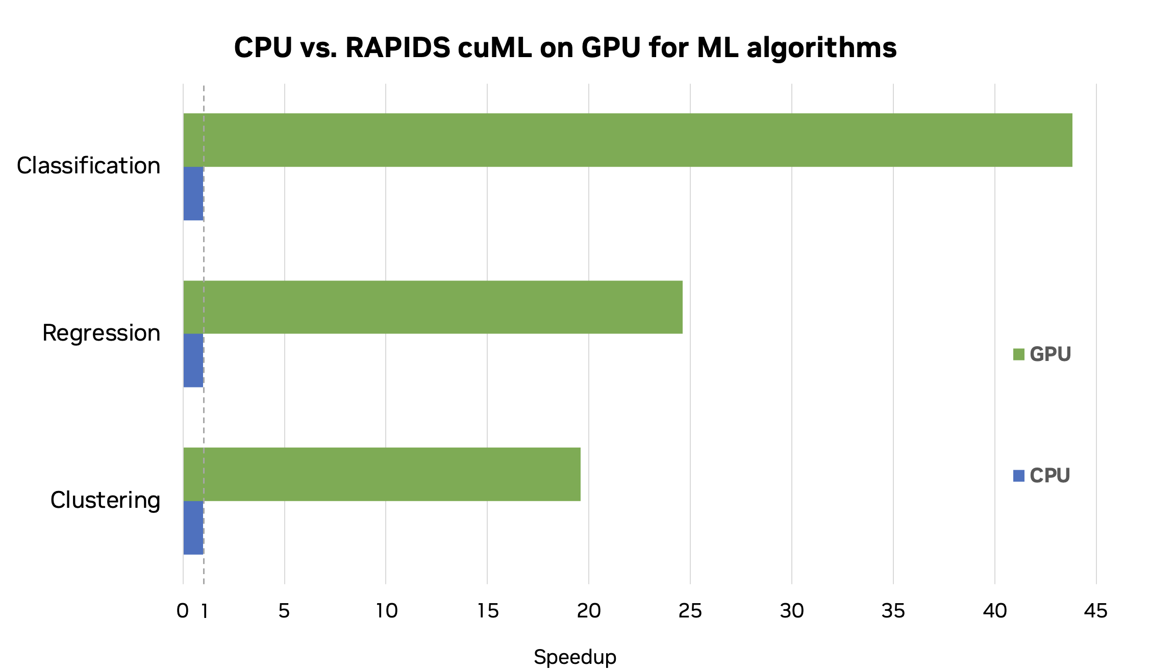
Benchmarking RAPIDS
This post is a simplified walkthrough of the complete workflow from the Introduction to Machine Learning Using cuML notebook on GitHub. This workflow resulted in a speedup of up to 44x for combined workflow of data loading, preprocessing, and ML training. These results were performed on an NVIDIA RTX 8000 GPU with RAPIDS 23.04 and Intel Core i7-7800X CPU.
Conclusion
GPU-accelerated machine learning with cuDF and cuML can drastically speed up your data science pipelines. With faster data preprocessing using cuDF and the cuML scikit-learn-compatible API, it is easy to start leveraging the power of GPUs for machine learning.
For a hands-on deep dive into the concepts discussed in this post, check out the Introduction to Machine Learning Using cuML notebook on GitHub. Learn more about GPU-accelerated data science workflows.
This post is part of a series on accelerated data analytics.
Update 11/20/2023: RAPIDS cuDF now comes with a pandas accelerator mode that allows you to run existing pandas workflow on GPUs with up to 150x speed-up requiring zero code change while maintaining compatibility with third-party libraries. The code in this blog still functions as expected, but we recommend using the pandas accelerator mode for seamless experience. Learn more about the new release in this TechBlog post.
