
A leading global retailer has invested heavily in becoming one of the most competitive technology companies around.
Accurate and timely demand forecasting for millions of item-by-store combinations is critical to serving their millions of weekly customers. Key to their success in forecasting is RAPIDS, an open-source suite of GPU-accelerated libraries. RAPIDS helps them tear through their massive-scale data and has improved forecasting accuracy by several percentage points. It now runs orders of magnitude faster on a reduced infrastructure GPU footprint. This enables them to respond in real-time to shopper trends and have more of the right products on the shelves, fewer out-of-stock situations, and increased sales.
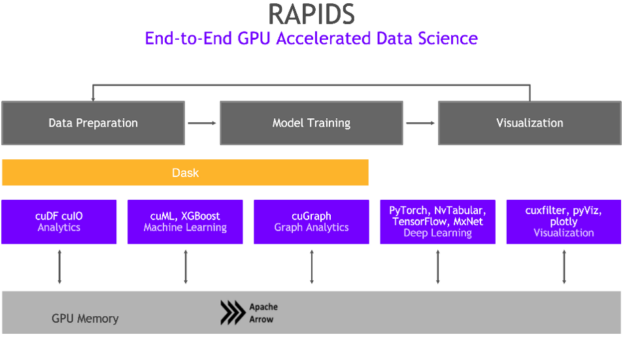
With RAPIDS, data practitioners can accelerate pipelines on NVIDIA GPUs, reducing data operations including data loading, processing, and training from days to minutes. RAPIDS abstracts the complexities of accelerated data science by building on and integrating with popular analytics ecosystems like PyData and Apache Spark, enabling users to see benefits immediately.
Compared to similar CPU-based implementations, RAPIDS delivers 50x performance improvements for classical data analytics and machine learning (ML) processes at scale, which drastically reduces the total cost of ownership (TCO) for large data science operations.
To learn and solve complex data science and AI challenges, leaders in retail often leverage what are called Kaggle competitions. Kaggle is a platform that brings together data scientists and other developers to solve challenging and interesting problems posted by companies. In fact, there have been over 20 competitions for solving retail challenges within the past year.
Leveraging RAPIDS and best practices for a forecasting competition, NVIDIA Kaggle Grandmaster Kazuki Onodera won 2nd place in the Instacart Market Basket Analysis Kaggle competition using complex feature engineering, gradient-boosted tree models, and special modeling of the competition’s F1 evaluation metric. Along the way, we documented the best practices for ETL, feature engineering, and building and customizing the best models for building an AI-based retail forecasting solution.
This post walks you through the components of a Kaggle competition to explain data science best practices for improving forecasting in retail. Specifically, the post explains the Instacart Market Basket Analysis Kaggle competition goals, introduces RAPIDS, then offers a workflow to show you how to explore the data visually, develop features, train the model, and run a forecasting prediction. Then, the post dives into some advanced techniques for feature engineering with model explainability and hyperparameter optimization (HPO).
- For an even more detailed look into the methodology, see Kazuki Onodera’s fantastic interview with Medium.com.
- Join Paul Hendricks at NVIDIA GTC 2021, where he hosts a session on Best Practices for ETL, Feature Engineering, and Model Development for Retail Forecasting Using NVIDIA RAPIDS Data Science Libraries.
- Access the Jupyter notebook where we share these best practices for GPU-accelerated forecasting within the context of the Instacart Market Basket Analysis Kaggle competition.
The forecasting challenge
The Instacart Market Basket Analysis competition challenged Kagglers to predict which grocery products a consumer will purchase again and when. Imagine, for example, having milk ready to be added to your cart right when you run out, or knowing that it’s time to stock up again on your favorite ice cream.
This focus on understanding temporal behavior patterns makes the problem fairly different from standard item recommendation, where user needs and preferences are often assumed to be relatively constant across short windows of time. Whereas Netflix might be fine with assuming you want to watch another movie like the one you just watched, it’s less clear that you’ll want to reorder a fresh batch of almond butter or toilet paper if you bought them yesterday.
Problem overview
The goal of this competition was to predict grocery reorders: given a user’s purchase history (a set of orders, and the products purchased within each order), which of their previously purchased products will they repurchase in their next order?
The problem is a little different from the general recommendation problem, where you often face a cold start issue of making predictions for new users and new items that you’ve never seen before. For example, a movie site may need to recommend new movies and make recommendations for new users.
The sequential and time-based nature of the problem also makes it interesting: how do you take the time since a user last purchased an item into account? Do users have specific purchase patterns and do they buy different kinds of items at different times of the day?
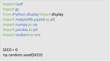
To get started, first load some of the modules you’ll be using in this notebook and set the random seed for any random number generator you’ll be using.
RAPIDS overview
Data scientists typically work with two types of data:
- Unstructured data often comes in the form of text, images, or videos.
- Structured data, as the name suggests, comes in a structured form, often represented by a table or CSV. We focus the majority of our tutorials on working with these types of data.
There are many tools in the Python ecosystem for structured, tabular data but few are as widely used as pandas. pandas represents data in a table and enables data scientists to manipulate the data to perform a number of useful operations, such as filtering, transforming, aggregating, merging, and visualizing. For more information, see the pandas documentation.
pandas is fantastic for working with small datasets that fit into your system’s memory. However, datasets are growing larger and data scientists are working with increasingly complex workloads. The need for accelerated compute power arises.
cuDF is a package within the RAPIDS ecosystem that allows data scientists to easily migrate existing pandas workflows from CPU to GPU, where computations can leverage the immense parallelization that GPUs provide.
Getting familiar with the data
The dataset for this competition contains several files capturing orders from Instacart users over time, with the goal of the competition to predict if a user will re-order a product and specifically, which products will they re-order.
From the Kaggle data description, you see that you have over three million grocery orders with a customer base of over 200,000 Instacart users. For each user, you are provided between 4 and 100 of their orders, with the sequence of products purchased in each order, as well as the time of their orders and a relative measure of time between orders. Also provided are the week and hour of the day the order was placed, and a relative measure of time between orders.
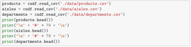
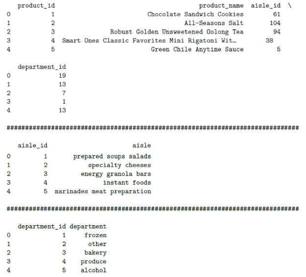
Your products, aisles, and departments datasets are composed of metadata about your products, aisles, and departments respectively. Each dataset (products, aisles, departments, and orders, and so on) has a unique identifier mapping for each entity in that dataset. For example, order_id represents a unique order within the orders dataset, product_id represents a unique product within the products dataset, and so on. You use these unique identifiers later to combine the separate datasets into one coherent view for exploratory data analysis, feature engineering, and modeling.
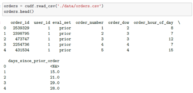
Next, you read in your data and inspect the different tables using cuDF.
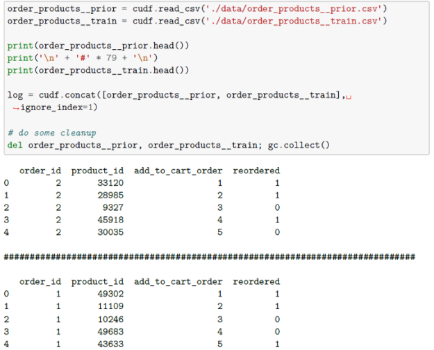
Additionally, you read in your orders datasets. The first indicates to which set (prior, train, test) an order belongs. Additional files specify which products were purchased in each order. Again, from the Kaggle description of the data, you see that the order_products__prior.csv contains previous order contents for all customers. The column reordered indicates that the customer has a previous order that contains the product. You are informed that some orders will have no reordered items.
Exploring the data
When you think about your data science workflow, one of the most important steps is exploratory data analysis. This is where you examine your data and look for clues and insights into which features you can use (or need to create) to feed your model.
There are many ways to explore the data and each exploratory data analysis is different for each problem. However, it still remains incredibly important as it informs your feature engineering process, ultimately determining how accurate your model will be.
In the notebook, you look at a couple different cross-sections of the day. Specifically, you examine the distribution of the order counts, the days of week and times customers typically place orders, the distribution of the number of days since the last order, and the most popular items across all orders and unique customers (de-duplicating so as to ignore customers who have a “favorite” item that they place repeated orders for).
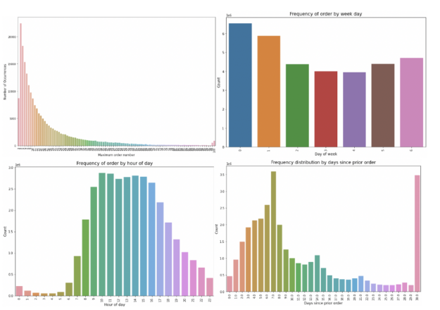
From this, you can see the following:
- There are no orders less than 4 and the max is capped at 100.
- The orders are high Saturday and Sunday (days 0 and 1) and low during Wednesday.
- The majority of orders are made during the daytime. And customers primarily order once a week or month (see the peaks at days 7 and 30).
For more information about similar exploratory analysis for product popularity, see Best Practices of Using AI to Develop the Most Accurate Retail Forecasting Solution.
Feature engineering
If exploratory data analysis is the most important part of the data science workflow, Feature engineering is a close second. This is where you identify which features should be fed into the model and create features where you believe they might be able to help the model do a better job of predicting.
Start by just identifying your unique User X Item combinations and sorting them. You create a dataset where each user maps to their most recent order number, day of week and hour, and how many days it’s been since that order. And you extend your dataset, creating labels and features to be used later in the machine learning model:
- How many kinds of products has the user ordered?
- How many products has the user ordered within one cart?
- From which departments has the user ordered products?
- When has the user ordered products (day of the week)?
- Has this user ordered this product at least once before?
- How many orders has a user placed that have included this item?
Solving for the business problem (train and predict)
The mathematical operations underlying many machine learning algorithms are often matrix multiplications. These types of operations are highly parallelizable and can be greatly accelerated using a GPU. RAPIDS makes it easy to build machine learning models in an accelerated fashion while still using a nearly identical interface to Scikit-Learn and XGBoost.
There are many ways to create a model. You can use linear regression models, SVMs, tree-based models like random forest and XGBoost, or even neural networks. In general, tree-based models tend to work better with tabular data for forecasting than neural networks. Neural networks work by mapping the input (feature space) to another complex boundary space and determining what values should belong to those points within that boundary space (regression, classification).
Tree-based models, on the other hand, work by taking the data, identifying a column, and then finding a split point in that column to map a value to, all the while optimizing the accuracy. You can create multiple trees using different columns, and even different columns within each tree. For more information about tree-based models XGBoost, see Introduction to Boosted Trees.
In addition to their better accuracy performance, tree-based models are very easy to interpret (important for when predictions or decisions resulting from the predictions must be explained and justified, maybe for compliance and legal reasons e.g. finance, insurance, healthcare). Tree-based models are very robust and work well even when there is a small set of data points.
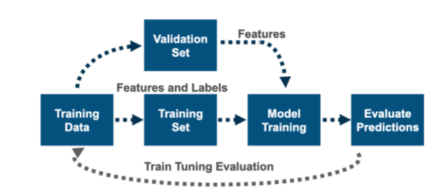
In the next section, you set the different parameters for your XGBoost model and train five different models, each on a different subset of users to avoid overfitting to a particular set of users.
import xgboost as xgb

NFOLD = 5
PARAMS = {
    'max_depth':8,
    'eta':0.1,
    'colsample_bytree':0.4,
    'subsample':0.75,
    'silent':1,
    'nthread':40,
    'eval_metric':'logloss',
    'objective':'binary:logistic',
    'tree_method':'gpu_hist'
         }

models = []
for i in range(NFOLD):
    train_ = train[train.user_id % NFOLD != i]
    valid_ = train[train.user_id % NFOLD == i]
    dtrain = xgb.DMatrix(train_.drop(['user_id', 'product_id', 'label'], axis=1), train_['label'])
    dvalid = xgb.DMatrix(valid_.drop(['user_id', 'product_id', 'label'], axis=1), valid_['label'])
    model = xgb.train(PARAMS, dtrain, 9999, [(dtrain, 'train'),(dvalid, 'valid')],
                      early_stopping_rounds=50, verbose_eval=5)
    models.append(model)
    break
There are several parameters that should be set before XGBoost can be run:
- General parameters relate to which booster you are using to do the boosting, commonly the tree or linear model.
- Booster parameters depend on which booster you have chosen.
- Learning task parameters decide on the learning scenario. For example, regression tasks may use different parameters with ranking tasks.
For more information about the configurable parameters within the XGBoost module, see XGBoost Parameters.
Feature importance
When you’ve trained your models, you might want to look at the internal workings and understand which of the features you’ve crafted are contributing the most to the predictions. This is called feature importance. One of the advantages for tree-based models for forecasting is that understanding the differing importance of your features is easy.
By understanding how the features contribute to the model accuracy, you can choose to remove features that aren’t important or try to iterate and create new features, re-train, and re-assess if those new features are more important.
Ultimately, being able to iterate quickly and try new things in this workflow leads to the most accurate model and the greatest ROI. For forecasting, ROI oftentimes comes from cost savings on reduced out-of-stock and poorly placed inventory.
Iteration traditionally can take a significant amount of time due to computational intensity. RAPIDS enables you to churn through model iteration with NVIDIA accelerated computing so that you can iterate quickly and determine the best-performing model.
In the Feature Importance section of the notebook, you define the convenience code to access the importance of the features in each model. You then pass in your list of models that you trained, iterate over them, and average the importance of each variable across all the models. Lastly, you visualize feature importance using a horizontal bar chart.
You see that three features are contributing the most to the predictions:
user_product_size: How many orders has a user placed that have included this item?user_product_t-1: Has this user ordered this product at least once before?order_number: The number of orders that the user has created.
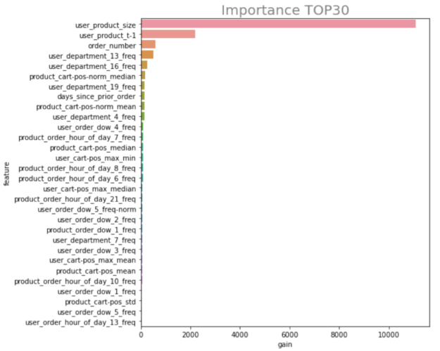
All this makes sense and aligns with your understanding of the problem. Customers who have placed an order for an item before are more likely to repeat an order for that product, and users who place multiple orders of that product are even more likely to re-order. The number of orders a customer has created correlates with their likelihood of re-ordering.
The code uses the default XGBoost implementation of feature importance, but you are free to choose any implementation or technique. A wonderful technique, also developed by an NVIDIA Kaggle Grandmaster Ahmet Erdem, is called LOFO.
Leave One Feature Out (LOFO) importance calculates the importance of a set of features based on a metric of choice, for a model of choice, by iteratively removing each feature from the set, and evaluating the performance of the model, with a validation scheme of choice, based on the chosen metric.
LOFO first evaluates the performance of the model with all the input features included, then iteratively removes one feature at a time, retrains the model, and evaluates its performance on a validation set. This methodology enables you to effectively determine which features are important for the model. LOFO has several advantages compared to other important types:
- It does not favor granular features.
- It generalizes well to unseen test sets.
- It is model agnostic.
- It gives negative importance to features that hurt performance upon inclusion.
For more information about LOFO, see Leave One Feature Out.
Hyperparameter optimization
When you trained the XGBoost models, you used the following parameters:
PARAMS = { 'max_depth':8, 'eta':0.1, 'colsample_bytree':0.4, 'subsample':0.75, 'silent':1, 'nthread':40, 'eval_metric':'logloss', 'objective':'binary:logistic', 'tree_method':'gpu_hist' }
Of these, only a few may be changed and affect the accuracy of the model: max_depth, eta, colsample_bytree, and subsample. However, these may not be the most optimal parameters. The art and science of identifying and training models with the model optimal hyperparameters is called hyperparameter optimization (HPO).
While there is no magic button one can press to automatically identify the most optimal hyperparameters, there are techniques that allow you to explore the range of all possible hyperparameter values, quickly test them, and find the values that are closest.
A full exploration of these techniques is beyond the scope of this notebook. However, RAPIDS is integrated into many Cloud ML Frameworks for doing HPO as well as with many of the different open source tools. And being able to use the incredible speedups from RAPIDS allows you to go through your ETL, feature engineering, and model training workflow very quickly for each possible experiment – ultimately resulting in fast HPO explorations through large hyperparameter spaces and a significant reduction in the total cost of ownership (TCO).
Conclusion
In this post, we walked through the components of a Kaggle competition to explain the data science best practices for improving forecasting in retail.
Specifically, we explained the Instacart Market Basket Analysis Kaggle competition goals, introduced RAPIDS, then offered a workflow to show how to explore the data visually, develop features, train the model, and run a forecasting prediction. We also reviewed techniques for feature engineering with model explainability and HPO.
For more information, see the following resources:
- Jupyter notebook on forecasting where we show best practices for GPU accelerated forecasting within the context of the Instacart Market Basket Analysis Kaggle competition in which NVIDIA Kaggle Grandmaster Kazuki Onodera won 2nd place, using complex feature engineering, gradient boosted tree models, and special modeling of the competition’s F1 evaluation metric.
- Join Paul Hendricks at NVIDIA GTC 2021, on Best Practices for ETL, Feature Engineering, and Model Development for Retail Forecasting Using NVIDIA RAPIDS Data Science Libraries.
- Read Kazuki Onodera’s detailed interview: Instacart Market Basket Analysis.
- See the Rapids.ai open-source website.
