At GTC Spring 2020, Adobe, Verizon Media, and Uber each discussed how they used Spark 3.0 with GPUs to accelerate and scale ML big data pre-processing, training, and tuning pipelines.
- Adobe Intelligent Services achieved a 7x performance improvement and 90 percent cost savings with a GPU-based Spark 3.0 and XGBoost intelligent email solution to optimize the delivery of marketing messages.
- Verizon Media built a distributed Spark ML pipeline for XGBoost model training and hyperparameter tuning on a GPU based cluster, to predict customer churn and achieved a 3x performance improvement compared to a CPU-based solution.
- Uber discussed how they are using Spark 3.0 with GPUs to have ETL and distributed deep learning training on GPUs within the same pipeline.
There are multiple challenges when it comes to the performance of large-scale machine learning (ML) solutions: huge datasets, complex data preprocessing and feature engineering pipelines, and model training and tuning.
One of the largest public datasets for recommendation tasks was used to demonstrate the efficiency of Spark-GPU data preprocessing and transformation for a deep learning pipeline. With eight V100 32-GB GPUs, processing time was sped up by a factor of up to 43X compared to an equivalent Spark-CPU pipeline. With GPUs having a significantly faster training speed over CPUs, data science teams can tackle larger data sets, iterate faster, and tune models more frequently to maximize prediction accuracy and business value.
This post walks you through using Apache Spark with GPUs to accelerate and optimize an end-to-end data exploration, ML, and hyperparameter tuning example to predict NYC taxi fares. We start with an overview of accelerating ML pipelines and XGBoost and then explore the use case.
GPU-accelerated end-to-end ETL and ML pipelines with Spark 3.0
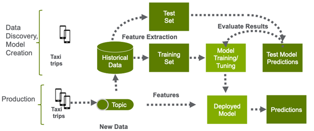
Supervised ML, also called predictive analytics, uses algorithms to train a model on finding patterns in a dataset with labels and features. It then uses the trained model to predict the labels on a new dataset’s features.
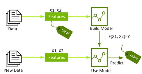
ML is an iterative, exploratory process that involves feature engineering, training, testing, and hyperparameter tuning ML algorithms before a model can be used in production to make predictions.
Feature engineering is the process of transforming raw data into inputs for an ML algorithm. With data science, you often hear about the algorithms that are used. However, a more significant part of a data scientist’s time —consuming about 80%—is taking the raw data and combining it in a way that is most predictive.
Hyperparameter optimization tunes the properties of the model that can be set for training, for example, the depth of a decision tree, to find the most accurate possible model for your problem.
GPUs have a massively parallel architecture consisting of thousands of small efficient cores designed for handling multiple tasks simultaneously. They have been responsible for advancing DL and ML model training in the past several years. However, data preprocessing was typically performed on CPUs.
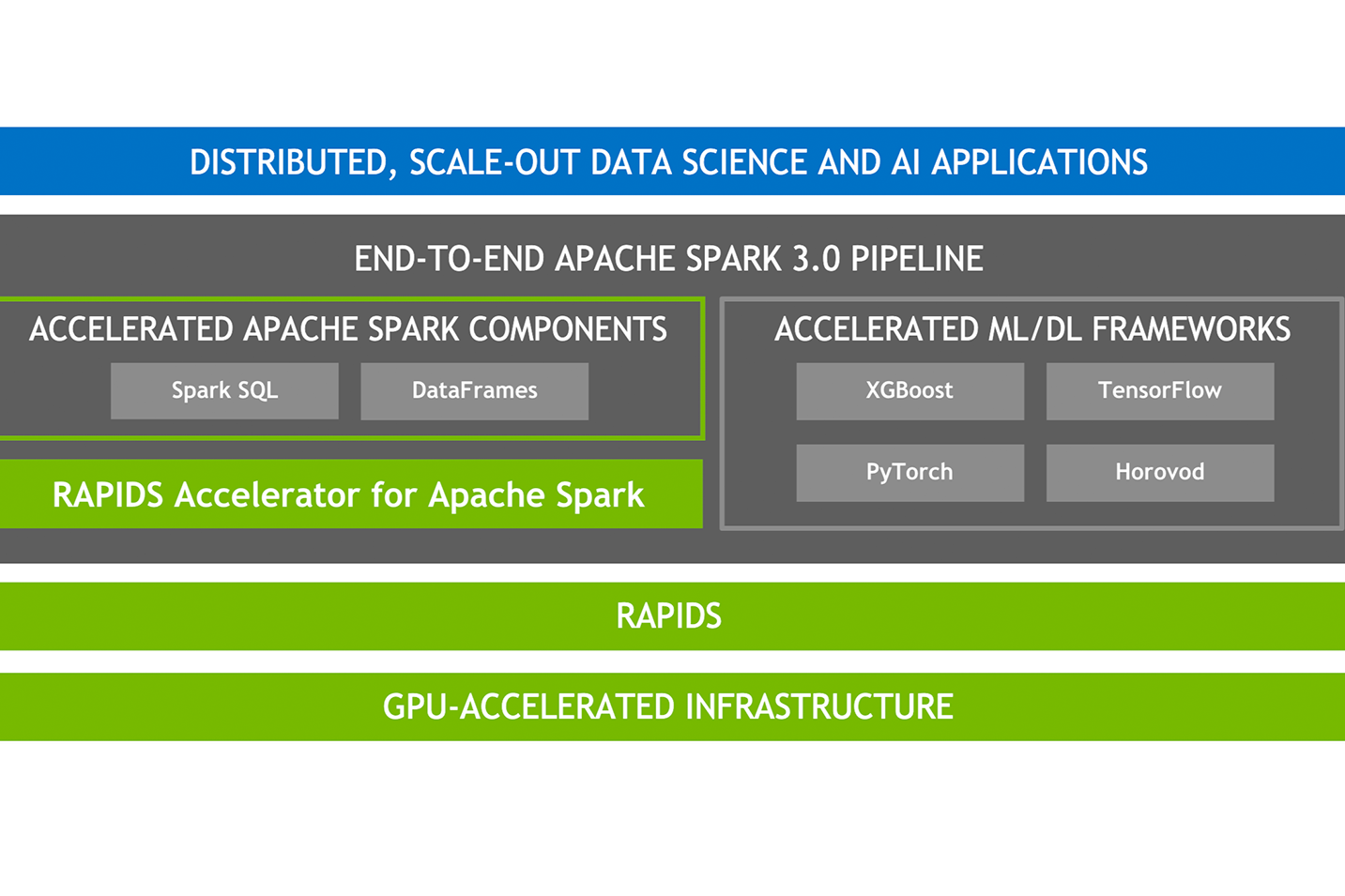
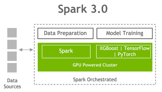
NVIDIA has been collaborating with the Apache Spark community to bring GPUs into Spark’s native processing. With Apache Spark 3.0 and the RAPIDS Accelerator for Apache Spark, you can now have a single pipeline, from data ingestion and data preparation to model training and tuning on a GPU-powered cluster. The RAPIDS Accelerator for Spark enables GPU-accelerated Spark SQL/DataFrame data processing and RAPIDS integration with XGBoost enables the GPU acceleration of XGBoost model training and tuning time.
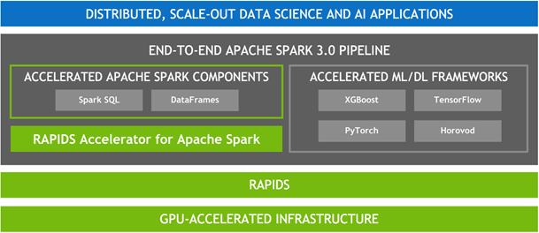
Growing ecosystem for accelerated Spark
Several leading Spark platforms can be accelerated with NVIDIA GPUs: Google Cloud, Databricks, and Cloudera.
In May 2020, Google Cloud announced the availability of Spark 3.0 preview on Dataproc image version 2.0, noting the powerful NVIDIA GPU acceleration that’s now possible thanks to the collaboration of the open source community. For more information, see Google Cloud and NVIDIA’s enhanced partnership accelerates computing workloads.
At SparkAISummit in June 2020, Databricks announced that Databricks Runtime 7.0 for Machine Learning features GPU-accelerator–aware scheduling with Spark 3.0, developed in collaboration with NVIDIA and other community members. It is also available on Microsoft Azure and AWS.
In his GTC 2020 keynote, NVIDIA CEO Jensen Huang revealed that NVIDIA and Cloudera are teaming up to accelerate the Cloudera Data Platform. Cloudera announced support for GPU-enabled Spark 3 and GPU-accelerated ML and DL frameworks and direct use of RAPIDS libraries in the Cloudera Data Platform (CDP) powered by NVIDIA. With a single, accelerated architecture, Cloudera customers can now run an end-to-end pipeline on-premises and in the cloud, all at 10x faster. This enables the following benefits:
- Incremental introduction of a Spark 3 and GPU infrastructure into your production environment, avoiding the need to “fork-lift upgrade” existing clusters
- Bursting from on-premises to cloud for additional resources
- Reducing development time in the cloud and deployment time on-premises from days to hours
Spark can also be run on-premises with the RAPIDS software and RAPIDS Accelerator for Spark being available directly from NVIDIA.
Overview of regression and XGBoost
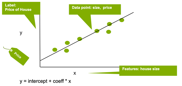
Regression estimates the relationship between a target outcome label and one or more feature variables to predict a continuous numeric value. In the following example, linear regression is used to estimate the house price (label) based on the house size (feature).
Decision trees create a model that predicts the label by evaluating a tree of if-then-else true/false feature questions and estimating the minimum number of questions needed to assess the probability of making a correct decision. Decision trees can be used for classification to predict a category or regression to predict a continuous numeric value.

Gradient boosting decision tree (GBDT) is an ensemble learning algorithm for classification and regression. GBDT uses a technique called boosting to iteratively build a model consisting of multiple shallow decision trees. The final prediction is a weighted average of all the decision tree predictions.
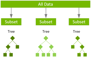
XGBoost, which stands for Extreme Gradient Boosting, is a leading, scalable, distributed variation of GBDT. With XGBoost, trees are built in parallel instead of sequentially like GBDT. XGBoost follows a level-wise strategy, scanning across gradient values and using these partial sums to evaluate the quality of splits at every possible split in the training set.
The RAPIDS team works closely with the DMLC XGBoost organization, and GPU-accelerated XGBoost now includes seamless, drop-in GPU acceleration, which significantly speeds up model training and improves accuracy. GPU-Accelerated Spark XGBoost speeds up the preprocessing of massive volumes of data, allows larger data sizes in GPU memory, and improves XGBoost training and tuning time.
Accelerating data transformation and exploration with Spark SQL
To build an ML model, you must clean, extract, explore, and test your dataset to find the features of interest that most contribute to the model’s accurate predictions. You can use Spark SQL to explore the public New York Taxi dataset and analyze the features that might help predict taxi fare amounts. In this example, you build a model to predict the taxi fare amount, based on the following:
- Label: Fare amount
- Possible features: {trip time, trip distance, pickup longitude, pickup latitude, rate code, dropoff longitude, dropoff latitude, hour, day of week}
Load the data from Parquet files into a Spark DataFrame, specifying the data source as shown in the code example. Cache the DataFrame so that Spark does not have to reload it for each query. Also, Spark can cache DataFrames or Tables in columnar format in memory.

var tdf = spark.read.parquet("dbfs:/taxi_data_parquet")
tdf.cache
tdf.createOrReplaceTempView("taxi")
Now you can use Spark DataFrames, SQL, Scala, and Python in the same notebook to explore and transform the data.
As shown in the following example, you can use Spark DataFrame transformations to discard columns that you won’t use, filter out anomalous or outlier values such as fare amounts below 0, and calculate the trip time. For more information about the complete code, see the nvidia/spark-rapids GitHub repo.
// drop unwanted columns
tdf=  tdf.drop("payment_type","extra")
// rename a column
tdf = tdf.withColumnRenamed("VendorID", "vendor_id")
// filter anomalous values
df = df.filter($"fare_amount" > 0 and $"fare_amount" < 100)
df = df.filter($"trip_distance" > 0 and $"trip_distance" < 100)
// calculate the trip time
df = df.withColumn("trip_time", unix_timestamp($"dropoff_time") -unix_timestamp($"pickup_time"))
After filtering and transforming the data, run a select * query or a DataFrame.show command to display the first rows of the taxi table.
%sql
select * from taxi

Now you can use Spark SQL to explore what might affect the taxi fare amount, with questions like, “What is the average fare amount and average trip distance by hour of the day?”
%sql
select hour, avg(fare_amount), avg(trip_distance)
from taxi
group by hour order by hour
With a Databricks, Zeppelin, or Jupyter notebook, you can display the SQL results in graph formats.
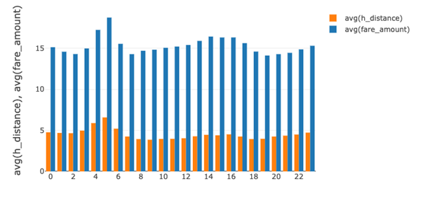
Here’s the same query with the DataFrame API:
df.groupBy("hour").avg("fare_amount", “h_distance”)
.orderBy("hour").show(5)
Here’s the result:
+----+------------------+-----------------+
|hour|  avg(fare_amount)|  avg(h_distance)|
+----+------------------+-----------------+
|   0| 15.12697411814677|4.769068352344985|
|   1| 14.57751020950744|4.686168090756313|
|   2|14.293304789803448| 4.65156782396335|
|   3|14.976290098512328|4.963535321742999|
+----+------------------+-----------------+
With Apache Spark 3.0, RAPIDS accelerator APIs are used by Spark SQL and DataFrames for GPU-accelerated, memory-efficient, columnar data processing and query plans. You can see the Spark SQL query physical plan for a DataFrame by calling the explain(“formatted”) method. In the following physical plan, you see that most operations are prefixed with Gpu. With the RAPIDS accelerator, the Catalyst query optimizer has been modified to identify operators within a query plan that can be accelerated with RAPIDS APIs, mostly a one-to-one mapping, and to schedule those operators on GPUs within the Spark cluster when executing the query plan.
tdf.groupBy("hour").avg("fare_amount", "h_distance").orderBy("hour").explain("formatted")
== Physical Plan ==
* GpuColumnarToRow (10)
+- GpuSort (9)
   +- GpuCoalesceBatches (8)
      +- GpuColumnarExchange (7)
         +- GpuHashAggregate (6)
            +- GpuCoalesceBatches (5)
               +- GpuColumnarExchange (4)
                  +- GpuHashAggregate (3)
                     +- HostColumnarToGpu (2)
                        +- InMemoryTableScan (1)
                              +- InMemoryRelation (2)
                                    +- * GpuColumnarToRow
(4)
                                       +- GpuScan parquet  (3)
You can use the Spark DataFrame describe function to perform summary statistics calculations on some numeric columns to understand the average and range for the label and important features.
tdf.select("passenger_count","h_distance","fare_amount","trip_time")
.describe().show
Here’s the result:
+-------+------------------+------------------+------------------+
|summary|        h_distance|       fare_amount|         trip_time|
+-------+------------------+------------------+------------------+
|  count|          24795119|          24795119|          24795119|
|   mean| 4.342987645673326|15.153788592421733|1009.6077538486506|
| stddev|4.1503010578443424|10.611002159248102|  695.290136980691|
|    min|               1.0|              1.01|                11|
|    max|            90.712|             99.99|             39997|
+-------+------------------+------------------+------------------+
The Spark DataFrame corr function can be used to measure the linear correlation between the label and features. In this example, the correlation between fare amount, trip distance, and trip time is .94 and .82, which is close to a total positive linear correlation of 1.
val dcor = tdf.stat.corr("fare_amount", "h_distance")
val tcor = tdf.stat.corr("fare_amount", "trip_time")
// result
0.9415
0.8163
Accelerating cross-validation training and hyperparameter optimization with grid search
To maximize the power of XGBoost to find the most accurate possible model, selecting the optimal hyperparameters is critical. The choice of optimal hyperparameters is in between underfitting and overfitting a model, where the model predictions match how the data behaves and are also generalized enough to predict on unseen data.
XGBoost has a lot of parameters to tune. For example, increasing the tree depth reduces underfitting and lowering the learning rate reduces overfitting. It could take you a long time to manually configure, test, and evaluate these options. This process can be accelerated and automated with Spark 3.0 GPUs and a training pipeline that tries out different combinations of parameters using a process called grid search, where you set up the hyperparameters to test in a cross-validation workflow.
Cross-validation tries out different combinations of hyperparameters to determine which values of the ML algorithm produce the best model. With cross-validation, the data is randomly split into k partitions. Each partition is used one time as the test dataset, while the rest are used for training. Models are then generated using the training sets and evaluated with the testing sets, resulting in k model accuracy measurements. The model hyperparameters leading to the highest accuracy measurements produce the best model.
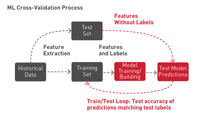
In this code example, you set up the XGBoostRegressor model estimator with the initial hyperparameters and features to train with. In this example, the features that you use are already in numeric format. With the CPU version of Spark XGBoost, the numeric features must be put into a feature vector with VectorAssembler. With the GPU version, just set the feature column to an array of feature column names.

// feature column names
val featureNames = Array("passenger_count","trip_distance", "pickup_longitude","pickup_latitude","rate_code","dropoff_longitude", "dropoff_latitude", "hour", "day_of_week","is_weekend")
// initial XGBoost hyperparameters
// for GPU version set the tree_method to gpu_hist
val regressorParam = Map(
    "learning_rate" -> 0.05,
    "gamma" -> 1,
    "objective" ->"reg:gamma",
    "subsample" -> 0.8,
    "num_round" -> 100,
    "tree_method" -> "gpu_hist")
// XGBoostRegressor Estimator to train the model
// for GPU version set the features column to feature names
val regressor = new XGBoostRegressor(regressorParam)
    .setLabelCol(“fare_amount”)
    .setFeaturesCols(featureNames)
The following code example sets up the CrossValidator with the grid of hyperparameters to test the model, the XGBoostRegressor estimator to train the model, and the RegressionEvaluator to evaluate the model. In the parameter grid, you test a max tree depth (maxDepth) of 3 and 8, with a learning rate (eta) of .2 and .6, giving four different parameter tests on three cross-validation partitions (NumFolds).
// grid of hyperparameters to test
val paramGrid = new ParamGridBuilder()
    .addGrid(regressor.maxDepth, Array(3, 8))
    .addGrid(regressor.eta, Array(0.2, 0.6))
    .build()
// Evaluator to test the model
var evaluator = new RegressionEvaluator()
    .setLabelCol(“fare_amount”)
// train the regressor, test with evaluator
// using parameter grid
val cv = new CrossValidator()
    .setEstimator(regressor)
    .setEvaluator(evaluator)
    .setEstimatorParamMaps(paramGrid)
    .setNumFolds(3)
The following code example uses the CrossValidator fit method on the training dataset to train and return the best XGBoostRegressor model from the cross-validation. On a Databricks cluster with 61.0 GB memory, 1 GPU, and 4.15 DBU, this training of 24,795,119 rows of data took 22 minutes, compared to 57 minutes on a CPU cluster with 61.0 GB memory, 8 cores, and 2 DBU. (This is not a benchmark.)

val cvmodel = cv.fit(tdf)
val model = cvmodel.bestModel.asInstanceOf[XGBoostRegressionModel]
The following code example gets the cross-validation for four hyperparameter metrics, which shows that the model with the best evaluation of RSME of 1.857 has an eta of .6 and maxDepth of 8.
cvmodel.getEstimatorParamMaps.zip(cvmodel.avgMetrics)
Array[(ParamMap, Double)] =
Array(({
     eta: 0.2,
     maxDepth: 3
},2.194134220469735), ({
     eta: 0.6,
     maxDepth: 3
},2.078462696071267), ({
     eta: 0.2,
     maxDepth: 8
},1.8857662413143166), ({
     eta: 0.6,
     maxDepth: 8
},1.857497448912559))
Evaluating the hyperparameter-tuned model
The performance of the model can be evaluated using the evaluation dataset, which has not been used for training. You get predictions on the evaluation data using the model transform method. The model estimates with the trained XGBoost model, and then returns the fare amount predictions in a new Predictions column of the returned DataFrame.

val edf = spark.read.parquet("dbfs:/eval_data_parquet")
pdf= model.transform(edf).cache()
pdf.select("fare_amount", "prediction").describe().show()
Here’s the result:
+-------+------------------+------------------+
|summary|       fare_amount|        prediction|
+-------+------------------+------------------+
|  count|           7440915|           7440915|
|   mean|15.154692854305472|15.154407281408535|
| stddev|10.620368305991281|10.455102375424485|
|    min|              1.11|0.8745052814483643|
|    max|             99.75|104.60748291015625|
+-------+------------------+------------------+
The RegressionEvaluator evaluate method calculates the root mean square error, which is the square root of the mean squared error, between the prediction and label columns. The result RMSE is 1.89, which is pretty good compared to an average fare amount of $15 with a standard deviation of 10.62. The R2 accuracy value that measures variation between the labels and predictions is .96, which is close to a perfect 1.

val rmse= evaluator.evaluate(pdf)
val r2 = evaluator.setMetricName("r2").evaluate(pdf)
Here’s the result:
RMSE == 1.8699602911729545
R2 == 0.9689982884556018
The model can be saved to disk to use later:
model.write.overwrite().save(savepath)
Reload the model with the load command:
val sameModel = XGBoostRegressionModel.load(savepath)
XGBoost Spark also supports saving the model to native format, to integrate it with other single-node libraries for further processing or for model serving on a single machine:
val nativeModelPath = "/tmp/nativeModel"
xgbClassificationModel.nativeBooster.saveModel(nativeModelPath)
Load this model with single-node Python XGBoost:
import xgboost as xgb
bst = xgb.Booster({'nthread': 4})
bst.load_model(nativeModelPath)
Conclusion
With GPU-Accelerated Spark and XGBoost, you can build fast data-processing pipelines, using Spark distributed DataFrame APIs for ETL and XGBoost for model training and hyperparameter tuning. With GPUs having a significantly faster training speed over CPUs, your data science teams can tackle larger data sets, iterate faster, and tune models more frequently to maximize prediction accuracy and business value.
- To access the RAPIDS Accelerator for Apache Spark and the getting started guide, visit the nvidia/spark-rapids GitHub repo.
- You can download the example code for this post and download the Spark XGBoost configuration and other Spark XGBoost examples.
- For more information about accelerating Apache Spark 3.0 with RAPIDS and GPUs, see Innovations to Accelerate Spark 3.0 Performance with GPUs and Accelerating Apache Spark 3.0 with GPUs.
- To dive even deeper into Apache Spark 3.0, download the free Apache Spark 3.0 ebook.
- To see a side-by-side comparison of the performance of a CPU cluster with that of a GPU cluster on the Databricks Platform, watch the Spark 3 Demo: Comparing Performance of GPUs vs. CPUs demo.
- View the NVIDIA GTC (GPU Technology Conference) session, Accelerating Cloudera Data Platform with NVIDIA RAPIDS.


